Chapter 16. Performance tips
In this chapter
- Key parameters of performance in actor systems
- Eliminating bottlenecks to improve performance
- Optimizing CPU usage with dispatcher tuning
- Changing the use of thread pools
- Performance improvements by changing thread releasing
We’ve pretty much run the gamut of Akka’s actor functionality thus far in the book. We started with structuring your applications to use actors, how to deal with state and errors, and how to connect with external systems and deal with persistence. You’ve also seen how you can scale out using clusters. We’ve used the Akka actors like a black box: you send messages to the ActorRef, and your receive method implementation is called with the message. The fact that you don’t need to know the internals of Akka is one of its biggest strengths. But there are times when you need more control over the performance metrics of an actor system. In this chapter we’ll show how you can customize and configure Akka to improve the overall performance.
Performance tuning is hard to do, and it’s different for every application. This is because the performance requirements vary, and all the components in a system will affect each other in different ways. The general approach is to find out which part is slow, and why. Based on the answer to those questions, find a solution. In this chapter we’ll focus on improving performance by configuring the threading backend that actors run on.
Here’s how the chapter progresses:
- First, a quick introduction to performance tuning and important performance metrics.
- Measuring the actors in a system by creating our own custom mailbox and an actor trait. Both implementations create statistical messages that enable us to find problem areas.
- The next step is to solve the problem area. We’ll start by describing the different options to improve one actor.
- But sometimes you just need to use resources more efficiently. In the last sections, we’ll focus on the use of threads. We’ll start with a discussion of how to detect that we have threading problems; after that, we’ll look at different solutions by changing the dispatcher configuration, which is used by the actors. Next we’ll describe how an actor can be configured to process many messages at a time on the same thread. Changing this configuration enables you to make a trade-off between fairness and increased performance.
- Finally, we’ll show how you can create your own dispatcher type for dynamically creating multiple thread pools.
To address performance problems, you need to understand how problems arise and how different parts interact with each other. When you understand the mechanism, you can determine what you need to measure to analyze your system, find performance problems, and solve them. In this section you’ll gain insight into how performance is affected, by determining which metrics are playing a key part in the system’s overall performance.
We’ll start by identifying the performance problem area of a system, followed by describing the most important performance metrics and terms.
Experience teaches that even though it’s difficult to see which of the many interacting parts of a system are limiting performance, it’s often only a small part affecting the system’s total performance. The Pareto principle (better known as the 80–20 rule) applies here: 80% of performance improvements can be made by addressing only 20% of the system. This is good and bad news. The good news is that it’s possible to make minor changes to the system to improve performance. The bad news is that only changes to that 20% will have any effect on the performance of the system. These parts that are limiting the performance of the whole system are called bottlenecks.
Let’s look at a simple example from chapter 8 where we created a pipes and filters pattern. We used two filters in a traffic camera example, which created the pipeline shown in figure 16.1.

When we look at this system, we can easily detect our bottleneck. The step “check license” can only service 5 images per second, while the first step can service 20 per second. Here we see that one step dictates the performance of the whole chain; therefore, the bottleneck of this system is the check-license step.
When our simple system needs to process two images per second, there isn’t a performance problem at all, because the system can easily process that amount and even has spare capacity. There will always be some part of the system that can be said to constrain performance, but it’s only a bottleneck if the amount the system is constrained exceeds an operational constraint on the business side.
So basically we keep on solving bottlenecks until we achieve our performance requirements. But there’s a catch. Solving the first bottleneck gives us the biggest improvement. Solving the next bottleneck will result in a lesser improvement (the concept of diminishing returns).
This is because the system will become more balanced with each change and reaches the limit of using all your resources. In figure 16.2 you see the performance reaching the limit when bottlenecks are removed. When you need a performance higher than this limit, you have to increase your resources, for example, by scaling out.

This, again, is one of the reasons why efforts should focus on requirements. One of the most common conclusions of metrics studies is that programmers tend to spend time optimizing things that have little effect on overall system performance (given the users’ experience). Akka helps address this by keeping the model closer to the requirements; we’re talking here about things that translate directly into the usage realm—licenses, speeders, and so on.
Thus far, we’ve been talking about performance in general, but there are two types of performance problems:
- The throughput is too low— The number of requests that can be served is too low, such as the capacity of the check-license step in our example.
- The latency is too long— Each request takes too long to be processed; for example, the rendering of a requested web page takes too long.
When having one of these problems, most people call it a performance problem. But the solutions to the problems can require vastly different amounts of time. Throughput problems are usually solved by scaling, but latency problems generally require design changes in your application. Solving performance problems of actors will be the focus of section 16.3, where we’ll show you how to improve performance by addressing bottlenecks. But first you need to learn a bit more about performance factors and parameters. You’ve just seen two of these: throughput and latency. We’ll cover these in more detail, and look also at other parameters. You’ll then have a good understanding of what can affect performance, before we address improving it in section 16.3.
Again, these are a function of the fact that our system is composed of actors and messages, not classes and functions, so we’re adapting what you already know about performance to the Akka realm.
Invariably, in the question of investigating the performance characteristics of a computer system, a lot of terms will make an appearance. We’ll start with a quick explanation of the most important ones. Then we’ll look at a single actor including the mailbox, as shown in figure 16.3. This figure shows the three most important performance metrics: arrival rate, throughput, and service time.

Let’s start with the arrival rate. This is the number of jobs or messages arriving during a period. For example, if eight messages were to arrive during our observation period of 2 seconds, the arrival rate would be four per second.
The next metric appeared in the previous section: the processing rate of the messages. This is called the throughput of the actor. The throughput is the number of completions during a period. Most will recognise this term, if not from prior performance tuning, then because network performance is measured in how many packets were successfully processed. As figure 16.4 shows, when a system is balanced, as it is at the top of the figure, it’s able to service all the jobs that arrive without making anyone wait. This means that the arrival rate is equal to the throughput (or at least doesn’t exceed it). When the service isn’t balanced, moving down in the figure, waiting invariably creeps in because the workers are all busy. In this way, message-oriented systems are really no different than thread pools (as you’ll see later).

In this case the node can’t keep up with the arrival of the messages, and the messages accumulate in the mailbox. This is a classic performance problem. It’s important to realize, though, that we don’t want to eliminate waiting; if the system never has any work waiting, we’ll end up with workers that are doing nothing. Optimal performance is right in the middle—each time a task is completed, there’s another one to do, but the wait time is vanishingly small.
The last parameter shown in figure 16.3 is the service time. The service time of a node is the time needed to process a single job. Sometimes the service rate is mentioned within these models. This is the average number of jobs serviced during a time period and is represented by μ. The relation between the service time (S) and service rate is this:
- μ = 1/S
The service time is closely related to the latency, because the latency is the time between the exit and the entry. The difference between the service time and the latency is the waiting time of a message in the mailbox. When the messages don’t need to wait in the mailbox for other messages to be completed, the service time is the latency.
The last performance term that’s often used within performance analysis is the utilization. This is the percentage of the time the node is busy processing messages. When the utilization of a process is 50%, the process is processing jobs 50% of the time and is idle 50% of the time. The utilization gives an impression of how much more the system can process, when pushed to the maximum. And when the utilization is equal to 100%, then the system is unbalanced or saturated. Why? Because if the demand grows at all, wait times will ensue immediately.
These are the most important terms pertaining to performance. If you paid attention, you noticed that the queue size is an important metric indicating that there’s a problem. When the queue size grows, it means that the actor is saturated and holding the entire system back.
Now that you know what the different performance metrics mean and their relations to each other, we can start dealing with our performance problems. The first step is to find the actors that have performance issues. In the next section, we’ll provide possible solutions to measure an actor system to find the bottlenecks.
Before you can improve the performance of the system, you need to know how it’s behaving. As you saw in section 16.1.1, you should only change the problem areas, so you need to know where the problem areas are. To do this, you need to measure your system. You’ve learned that growing queue sizes and utilization are important indicators of actors with performance problems. How can you get that information from your application? In this section we’ll show you an example of how to build your own means for measuring performance.
Looking at the metrics queue sizes and utilization, you see that you can divide the data into two components. The queue sizes have to be retrieved from the mailbox, and the utilization needs the statistics of the processing unit. In figure 16.5 we show the interesting times when a messages is sent to an actor and is processed.

When you translate this to your Akka actors, you need the following data (from the Akka mailbox):
- When a message is received and added to the mailbox
- When it was sent to be processed, removed from the mailbox, and handed over to the processing unit
- When the message was done processing and left the processing unit
When you have these times for each message, you can get all the performance metrics you need to analyze your system. For example, the latency is the difference between the arrival time and the leaving time. In this section we’ll create an example that retrieves this information. We’ll start by making our own custom mailbox that retrieves the data needed to trace the message in the mailbox. In the second part, we’ll create a trait to get the statistics of the receive method. Both examples will send statistics to the Akka EventStream. Depending on our needs, we could just log these messages or do some processing first. We don’t describe in the book how to collect these statistics messages, but with the knowledge you have now, it isn’t hard to implement by yourself.
Micro benchmarking
A common problem with finding performance problems is how to add code measurements that won’t affect the performance you’re trying to measure.
Just like adding println statements to your code for debugging, measuring timestamps with System.currentTimeMillis is a simple way to get a rough indicator to the problem in many cases. In other cases it falls short entirely.
Use a micro benchmarking tool like JMH (http://openjdk.java.net/projects/code-tools/jmh/) when more fine-grained performance testing is required.
From the mailbox, we want to know the maximum queue size and the average waiting time. To get this information, we need to know when a message arrives in the queue and when it leaves. First, we’ll create our own mailbox. In this mailbox, we’ll collect data and send it using the EventStream to one actor that processes the data into the performance statistics we need for detecting bottlenecks.
To create a custom queue and use it, we need two parts. The first is a message queue that will be used as the mailbox, and the second is a factory class that creates a mailbox when necessary. Figure 16.6 shows the class diagram of our mailbox implementation.

The Akka dispatcher is using a factory class (MailboxType) to create new mailboxes. By switching the MailboxType, we’re able to create different mailboxes. When we want to create our own mailbox, we’ll need to implement a MessageQueue and a MailboxType. We’ll start with mailbox creation.
- def enqueue(receiver: ActorRef, handle: Envelope)—This method is called when trying to add an Envelope. The Envelope contains the sender and the actual message.
- def dequeue(): Envelope—This method is called to get the next message.
- def numberOfMessages: Int—This returns the current number of messages held in this queue.
- def hasMessages: Boolean—This indicates whether this queue is non-empty.
- def cleanUp(owner: ActorRef, deadLetters: MessageQueue)—This method is called when the mailbox is disposed of. Normally it’s expected to transfer all remaining messages into the dead-letter queue.
We’ll implement a custom MonitorQueue which will be created by a MonitorMailboxType. But first we’ll define the case class containing the trace data needed to calculate the statistics, called MailboxStatistics. We’ll also define a class used to contain the trace data while collecting the data, MonitorEnvelope, while the message is waiting in the mailbox, as shown in the next listing.
The class MailboxStatistics contains the receiver, which is the actor that we’re monitoring. entryTime and exitTime contain the time the message arrived or left the mailbox. Actually we don’t need the queueSize, because we can calculate it from the statistics, but it’s easier to add the current stack size too.
In the MonitorEnvelope, the handle is the original Envelope received from the Akka framework. Now we can create the MonitorQueue.
The constructor of the MonitorQueue will take a system parameter so we can get to the eventStream later, which is shown in listing 16.2. We also need to define the semantics that this queue will support. Since we want to use this mailbox for all actors in the system, we’re adding the UnboundedMessageQueueSemantics and the LoggerMessageQueueSemantics. The latter is necessary since actors used internally in Akka for logging requires these semantics.
Selecting a Mailbox with specific Message Queue semantics
The semantics traits are simple marker traits (they do not define any methods). In this use case we don’t need to define our own semantics, though it can be convenient in certain cases, since an actor can require a specific semantics by using a RequiresMessageQueue; for instance, the DefaultLogger requires LoggerMessageQueueSemantics by mixing in a RequiresMessageQueue[LoggerMessageQueueSemantics] trait. You can link a mailbox to semantics using the akka.actor.mailbox.requirements configuration setting.
Next we’ll implement the enqueue method, which creates a MonitorEnvelope and adds it to the queue.
The queueSize is the current size plus one, because this new message isn’t added to the queue yet. Then we set about implementing the dequeue method. dequeue checks if the polled message is a MailboxStatistics instance, in which case it skips it, since we want to use the MonitorQueue for all mailboxes, and if we don’t exclude these messages, this will recursively create MailboxStatistics messages when it’s used by our statistics collector.
The next listing shows the implementation of the dequeue method.
When we’re processing a normal message, we create a MailboxStatistics and publish it to the EventStream. When we don’t have any messages, we need to return null to indicate that there aren’t any messages. At this point we’ve implemented our functionality, and all that’s left is to implement the other supporting methods defined in the MessageQueue trait.
Our mailbox trait is ready to be used in the factory class, described in the next section.
The factory class, which creates the actual mailbox, implements the MailboxType trait. This trait has only one method, but we also need a specific constructor, so this should also be considered as part of the interface of the MailboxType. Then the interface becomes this:
- def this(settings: ActorSystem.Settings, config: Config)—This is the constructor used by Akka to create the MailboxType.
- def create(owner: Option[ActorRef], system: Option[ActorSystem]): MessageQueue—This method is used to create a new mailbox.
When we want to use our custom mailbox, we need to implement this interface. Our fully implemented MailboxType is shown next.
When we don’t get an ActorSystem, we throw an exception because we need the ActorSystem to be able to operate. Now we’re done implementing the new custom mailbox. All that’s left is to configure the Akka framework that it will use as its mailbox.
When we want to use another mailbox, we can configure this in the application.conf file. There are multiple ways to use the mailbox. The type of the mailbox is bound to the dispatcher used, so we can create a new dispatcher type and use our mailbox. This is done by setting the mailbox-type in the application.conf configuration file, and we use the dispatcher when creating a new actor. One way is shown in the following snippet:
We mentioned before that there are other ways to get Akka to use our mailbox. The mailbox is still bound to the chosen dispatcher, but we can also overrule which mailbox the default dispatcher should use, with the result that we don’t have to change the creation of our actors. To change the mailbox used by the default dispatcher, we can add the following lines in the configuration file:
This way, we use our custom mailbox for every actor. Let’s see if everything is working as designed.
To test the mailbox, we need an actor that we can monitor. Let’s create a simple one. It does a delay before receiving a message, to simulate the processing of the message. This delay simulates the service time of our performance model.
Now that we have an actor to monitor, let’s send some messages to this actor.
As you can see, we get a MailboxStatistics for each message sent on the EventStream. At this point, we have completed the code to be able to trace the mailbox of our actors. We’ve created our own custom mailbox to put the tracing data of the mailbox on the EventStream, and learned that we need a factory class and the mailbox type to be able to use the mailbox. In the configuration we can define which factory class has to be used when creating a mailbox for a new actor. Now that we can trace the mailbox, let’s turn our attention to the processing of messages.
The data we need for tracing performance can be retrieved by overriding the actor’s receive method. This example requires the receive method of an actor to be changed for monitoring it, which is more intrusive than the mailbox example, because we have the ability to add the functionality without changing the original code. To be able to use the next example, we need to add the trait with every actor we want to trace. Again we start by defining the statistics message:
The receiver is the actor we monitor, and our statistics contain the entry and exit times. We also add the sender, which can give more information on the messages processed, but we’re not using this in these examples. Now that we have our ActorStatistics, we can implement the functionality by creating the trait that overrides the receive method.
We use the abstract override to get in between the actor and the Akka framework. This way we can capture the start and end time of processing the message. When the processing is done, we create the ActorStatistics and publish it to the event stream.
To do this, we can simply mixin the trait when creating the actor:
When we send a message to the ProcessTestActor, we expect an ActorStatistics message on the EventStream.
And just as expected, the processing time (exit time minus entry time) is close to the set service time of our test actor.
At this point we’re also able to trace the processing of the messages. We now have a trait that creates the tracing data and distributes that data using the EventStream. Now we can start to analyze the data and find our actors with performance issues. When we’ve identified our bottlenecks, we’re ready to solve them. In the next sections, we’ll look at different ways to address those bottlenecks.
To improve the system’s performance, you only have to improve the performance of the bottlenecks. There are a variety of solutions, but some have more impact on throughput, and others more directly impact latency. Depending on your requirements and implementation, you can choose the solution best suited to your needs. When the bottleneck is a resource shared between actors, you need to direct the resource to the tasks most critical for your system and away from tasks that aren’t that critical and can wait. This tuning is always a trade-off. But when the bottleneck isn’t a resource problem, you can make changes to your system to improve performance.
When you look at a queueing node in figure 16.7, you see that it contains two parts: the queue and the processing unit. You’ll also note the two performance parameters we just explored in section 16.1.2: arrival rate and the service time. We added a third parameter to add more instances of an actor: the number of services. This is actually a scaling-up action. To improve the performance of an actor, you can change three parameters:
- Number of services— Increasing the number of services increases the possible throughput of the node.
- Arrival rate— Reducing the number of messages to be processed makes it easier to keep up with the arrival rate.
- Service time— Making processing faster improves latency and makes it possible to process more messages, which also improves the throughput.

When you want to improve performance, you have to change one or more of these parameters. The most common change is to increase the number of services. This will work when throughput is a problem, and the process isn’t limited by the CPU. When the task uses a lot of CPU, it’s possible that adding more services could increase the service times. The services compete for CPU power, which can decrease the total performance.
Another approach is reducing the number of tasks that need to be processed. This approach is often forgotten, but reducing the arrival rate can be an easy fix that can result in a dramatic improvement. Most of the time, this fix requires changing the design of the system. But this doesn’t have to be a hard thing to do. In section 8.1.2 on the pipes and filters pattern, you saw that simply changing the order of two steps can make an impressive improvement in performance.
The last approach is to reduce service time. This will increase throughput and decrease response time, and will always improve performance. This is also the hardest to achieve, because the functionality has to be the same, and most of the time it’s hard to remove steps to reduce service time. One thing worth checking is if the actor is using blocking calls. This will increase service time, and the fix is often easy: rewrite your actor to use nonblocking calls by making it event-driven. Another option to reduce service time is to parallelize the processing. Break up the task and divide it over multiple actors, and make sure that tasks are processed in parallel by using, for example, the scatter-gather pattern, explained in chapter 8.
But there are also other changes that can improve performance, for example, when server resources like CPU, memory, or disk usage are the problem. If utilization of these resources is 80% or more, they’re probably holding your system back. This can be because you use more resources than you have available, which can be solved by buying bigger and faster platforms, or you can scale out. This approach would also require a design change, but with Akka scaling out doesn’t need to be a big problem, as we’ve shown in chapter 13 using clusters.
But resource problems don’t always mean that you need more. Sometimes you need to use what you have more sensibly. For example, threads can cause issues when you use too many or too few. This can be solved by configuring the Akka framework differently and using available threads more effectively. In the next section, you’ll learn how to tune Akka’s thread pools by assigning one thread to each task, which eliminates the repeated context-switch of the thread.
In chapter 1 we mentioned that the dispatcher of an actor is responsible for assigning threads to the actor when there’s a message waiting in the mailbox. Until now you didn’t need to know about the details of the dispatcher (although we changed the behavior earlier in chapter 9 with the routers). Most of the time, the dispatcher instance is shared between multiple actors. It’s possible to change the configuration of the default dispatcher or create a new dispatcher with a different configuration. In this section we’ll start by figuring out how to recognize a thread pool problem. Next, we’ll create a new dispatcher for a group of actors. And after that we’ll show how you can change the thread pool size and how to use a dynamically sized thread pool by using another executor.
In chapter 9 you saw that you can change the behavior of actors by using the Balancing-Dispatcher. But there are more configuration changes we can make to the default dispatcher that will affect performance. Let’s start with a simple example. Figure 16.8 shows a receiver actor and 100 workers.

The receiver has a service time of 10 ms, and there are 100 workers with a service time of 1 second. The maximum throughput of the system is 100/s. When we implement this example in Akka, we get some unexpected results. We use an arrival rate of 66 messages/s, which is below the 80% threshold we discussed. The system shouldn’t have any problems keeping up. But when we monitor it, we see that the queue size of the receiver is increasing over time (as column 2 of table 16.1 shows).
Table 16.1. Monitor metrics of the test example
| Period number |
Receiver: Max mailbox size |
Receiver: Utilization |
Worker 1: Max mailbox size |
Worker 1: Utilization |
|---|---|---|---|---|
| 1 | 70 | 5% | 1 | 6% |
| 2 | 179 | 8% | 1 | 6% |
| 3 | 285 | 8% | 1 | 10% |
| 4 | 385 | 7% | 1 | 6% |
According to these numbers, the receiver can’t process the messages before the next message arrives, which is strange because the service time is 10 ms, and the time between the messages is 15 ms. What’s happening? You learned from our discussion of performance metrics that when an actor is the bottleneck, the queue size increases and the utilization approaches 100%. But in our example, you see the queue size is growing but the utilization is still low at 6%. This means that the actor is waiting for something else. The problem is the number of threads available for the actors to process. By default, the number of threads available is three times the number of available processors within your server, with a minimum of 8 and a maximum of 64 threads. In this example we have a two-core processor, so there are 8 threads available (minimum number of threads). During the time that 8 workers are busy processing messages, the receiver has to wait until one worker has finished before it can process the waiting messages.
How can we improve this performance? The actor’s dispatcher is responsible to give the actor a thread when there are messages. To improve this situation, we need to change the configuration of the dispatcher used by the actors.
The behavior of the dispatcher can be changed by changing its configuration or dispatcher type. Akka has four built-in types, as shown in table 16.2.
Table 16.2. Available built-in dispatchers
| Type |
Description |
Use case |
|---|---|---|
| Dispatcher | This is the default dispatcher, which binds its actors to a thread pool. The executor can be configured, but uses the fork-join-executor as default. This means that it has a fixed thread pool size. | Most of the time, you’ll use this dispatcher. In almost all our previous examples, we used this dispatcher. |
| PinnedDispatcher | This dispatcher binds an actor to a single and unique thread. This means that the thread isn’t shared between actors. | This dispatcher can be used when an actor has a high utilization and has a high priority to process messages, so it always needs a thread and can’t wait to get a new thread. But you’ll see that usually better solutions are available. |
| BalancingDispatcher | This dispatcher redistributes the messages from busy actors to idle actors. | We used this dispatcher in the router load-balancing example in section 9.1.1. |
| CallingThreadDispatcher | This dispatcher uses the current thread to process the messages of an actor. This is only used for testing. | Every time you use TestActorRef to create an actor in your unit test, this dispatcher is used. |
When we look at our receiver actor with 100 workers, we could use the Pinned-Dispatcher for our receiver. This way it doesn’t share the thread with the workers. And when we do, it solves the problem of the receiver being the bottleneck. Most of the time a PinnedDispatcher isn’t a solid solution. We used thread pools in the first place to reduce the number of threads and use them more efficiently. In our example the thread will be idle 33% of the time if we use a PinnedDispatcher. But the idea of not letting the receiver compete with the workers is a possible solution. To achieve this, we give the workers their own thread pool by using a new instance of the dispatcher. This way we get two dispatchers, each with its own thread pool.
We’ll start by defining the dispatcher in our configuration, and using this dispatcher for our workers.
When we do the same test as before, we get the results shown in table 16.3.
Table 16.3. Monitoring metrics of the test example using a different thread pool for the workers
| Period number |
Receiver: Max mailbox size |
Receiver: Utilization |
Worker 1: Max mailbox size |
Worker 1: Utilization |
|---|---|---|---|---|
| 1 | 2 | 15% | 1 | 6% |
| 2 | 1 | 66% | 2 | 0% |
| 3 | 1 | 66% | 5 | 33% |
| 4 | 1 | 66% | 7 | 0% |
We see that the receiver is now performing as expected and is able to keep up with the arriving messages, because the maximum queue size is 1. This means that the previous message was removed from the queue before the next one arrived. And when we look at the utilization, we see that it is 66%, exactly what we expect: every second we process 66 messages that take 10 ms each.
But now the workers can’t keep up with the arriving messages, as indicated by column 5. Actually, we see that there are periods when the worker isn’t processing any message during the measurement period (utilization is 0%). By using another thread pool, we only moved the problem from the receiver to the workers. This happens a lot when tuning a system. Tuning is usually a trade-off. Giving one task more resources means that other tasks get less. The trick is to direct the resources to the most critical tasks for your system, away from tasks that are less critical and can wait. Does this mean we can’t do anything to improve this situation? Do we have to live with this result?
In our example we see that the workers can’t keep up with the arrival of messages, which is caused because we have too few threads, so why don’t we increase the number of threads? We can, but the result greatly depends on how much CPU the workers need to process a message.
Increasing the number of threads will have an adverse effect on the total performance when the processing is heavily dependent on CPU power, because one CPU core can only execute one thread at any given moment. When it has to service multiple threads, it has to switch context between multiple threads. This context switch also takes CPU time, which reduces the time used to service the threads. When the ratio of number of threads to available CPU cores becomes too large, the performance will only decrease. Figure 16.9 shows the relationship between the performance and number of threads for a given number of CPU cores.
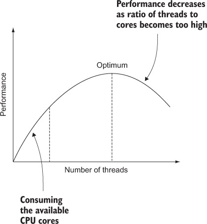
The first part of the graph (up to the first dotted vertical line) is almost linear, until the number of threads is equal to the number of available cores. When the number of threads increases even more, the performance still increases, but at a slower rate until it reaches the optimum. After that, the performance decreases when the number of threads increases. This graph assumes that all the available threads need CPU power. So there’s always an optimum number of threads. How can you know if you can increase the number of threads? Usually the utilization of the processors can give you an indication. When this is 80% or higher, increasing the number of threads will probably not help to increase the performance.
But when the CPU utilization is low, you can increase the number of threads. In this case the processing of messages is mainly waiting. The first thing you should do is check whether you can avoid the waiting. In this example it looks like freezing your actor and not using nonblocking calls, for example, using the ask pattern, would help. When you can’t solve the waiting problem, it’s possible to increase the number of threads. In our example we’re not using any CPU power, so let’s see in our next configuration example if increasing the thread number works.
The number of used threads can be configured with three configuration parameters in the dispatcher configuration:
The number of threads used is the number of available processors multiplied by the parallelism-factor, but with a minimum of parallelism-min and a maximum of parallelism-max. For example, when we have an eight-core CPU, we get 24 threads (8 × 3). But when we have only two cores available, we get 8 threads, although the number would be 6 (2 × 3), because we’ve set a minimum of 8.
We want to use 100 threads independent of the number of cores available; therefore, we set the minimum and maximum to 100:
Finally, when we run the example, we can process all the received messages in time. Table 16.4 shows that with the change, the workers also have a utilization of 66% and a queue size of 1.
Table 16.4. Monitoring metrics of the test example using 100 threads for the workers
| Period number |
Receiver: Max mailbox size |
Receiver: Utilization |
Worker 1: Max mailbox size |
Worker 1: Utilization |
|---|---|---|---|---|
| 1 | 2 | 36 | 2 | 34 |
| 2 | 1 | 66 | 1 | 66 |
| 3 | 1 | 66 | 1 | 66 |
| 4 | 1 | 66 | 1 | 66 |
| 5 | 1 | 66 | 1 | 66 |
In this case we could increase the performance of our system by increasing the number of threads. In this example we used a new dispatcher for only the workers. This is better than changing the default dispatcher and increasing the number of threads, because normally this is just a small part of the complete system, and when we increase the number of threads, it’s possible that 100 other actors will run simultaneously. And it’s possible that the performance will drop drastically because these actors depend on CPU power, and the ratio between active threads and CPU cores is out of balance. When using a separate dispatcher, only the workers run simultaneously in large numbers, and the other actors use the default available threads.
In this section you’ve seen how you could increase the number of threads, but there are situations when you want to change the thread size dynamically, for example, if the worker load changes drastically during operation time. This is also possible with Akka, but we need to change the executor used by the dispatcher.
In the previous section, we had a static number of workers. We could increase the number of threads, because we knew how many workers we had. But when the number of workers depends on the system’s work load, you don’t know how many threads you need. For example, suppose we have a web server, and for each user request a worker actor is created. The number workers depends on the number of concurrent users on the web server. We could handle this by using a fixed number of threads, which works perfectly most of the time. The important question is this: what size do we use for the thread pool? When it’s too small, we get a performance penalty, because requests are waiting for each other to get a thread, like the first example of the previous section, shown in table 16.1. But when we make the thread pool too big, we’re wasting resources. This is again a trade-off between resources and performance. But when the number of workers is normally low or stable but sometimes increases drastically, a dynamic thread pool can improve performance without wasting resources. The dynamic thread pool increases in size when the number of workers increases, but decreases when the threads are idle too long. This will clean up the unused threads, which otherwise would waste resources.
To use a dynamic thread pool, we need to change the executor used by the dispatcher. This is done by setting the executor configuration item of the dispatcher configuration. There are three possible values for this configuration item, as shown in table 16.5.
Table 16.5. Configuring executors
When you need a dynamic thread pool, you need to use the thread-pool-executor, and this executor also has to be configured. The default configuration is shown in the next code listing.
The minimum and maximum thread pool sizes are calculated, as can be seen in the fork-join-executor in section 16.4.1. When you want to use a dynamic thread pool, you need to set the task-queue-size. This will define how quickly the pool size will grow when there are more thread requests than threads. By default it’s set to -1, indicating that the queue is unbounded and the pool size will never increase. The last configuration item we want to address is the keep-alive-time. This is the idle time before a thread will be cleaned up, and it determines how quickly the pool size will decrease.
In our example we set the core-pool-size close to or just below the normal number of threads we need, and set the max-pool-size to a size where the system is still able to perform, or to the maximum supported number of concurrent users.
You’ve seen in this section how you can influence the thread pool used by the dispatcher that assigns threads to an actor. But there’s another mechanism that’s used to release the thread and give it back to the thread pool. By not returning the thread when an actor has more messages to process, you eliminate waiting for a new thread and the overhead of assigning a thread. In busy applications this can improve the overall performance of the system.
In previous sections you saw how you can increase the number of threads, and that there’s an optimum number, which is related to the number of CPU cores. When there are too many threads, the context switching will degrade performance. A similar problem can arise when different actors have a lot of messages to process. For each message an actor has to process, it needs a thread. When there are a lot of messages waiting for different actors, the threads have to be switched between the actors. This switching can also have a negative influence on performance.
Akka has a mechanism that influences the switching of threads between actors. The trick is not to switch a thread after each message when there are messages still in the mailbox waiting to be processed. A dispatcher has a configuration parameter, throughput, and this parameter is set to the maximum number of messages an actor may process before it has to release the thread back to the pool:
The default is set to 5. This way the number of thread switches is reduced, and overall performance is improved.
To show the effect of the throughput parameter, we’ll use a dispatcher with four threads and 40 workers with a service time close to zero. At the start, we’ll give each worker 40,000 messages, and we’ll measure how much time it takes to process all the messages. We’ll do this for several values of throughput. The results are shown in figure 16.10.

As you can see, increasing the throughput parameter will improve performance because messages are processed faster.[1]
1The Akka “Let it crash” blog has a nice post on how to process 5 million messages per second by changing the throughput parameter: http://letitcrash.com/post/20397701710/50-million-messages-per-second-on-a--single-machine.
In these examples we have better performance when we set the parameter high, so why is the default 5 and not 20? This is because increasing throughput also has negative effects. Let’s suppose we have an actor with 20 messages in its mailbox, but the service time is high, for example, 2 seconds. When the throughput parameter is set to 20, the actor will claim the thread for 40 seconds before releasing the thread. Therefore, other actors wait a long time before they can process their messages. In this case the benefit of the throughput parameter is less when the service time is greater, because the time it takes to switch threads is far less than the service time, which can be negligible. The result is that actors with a high service time can take the threads for a long time. For this there’s another parameter, throughput-deadline-time, which defines how long an actor can keep a thread even when there are still messages and the maximum throughput hasn’t been reached yet:
By default, this parameter is set to 0ms, meaning that there isn’t a deadline. This parameter can be used when you have a mix of short and long service times. An actor with a short service time processes the maximum number of messages after obtaining a thread, while an actor with a long service time will only process one message or multiple messages until it reaches 200 ms each time it obtains a thread.
Why can’t we use these settings as our default? There are two reasons. The first one is fairness. Because the thread isn’t released after the first message, the messages of other actors need to wait longer to be processed. For the system as a whole, this can be beneficial, but for individual messages, it can be a disadvantage. With batch-like systems, it doesn’t matter when messages are processed, but when you’re waiting for a message, for instance, one that’s used to create a web page, you don’t want to wait longer than your neighbor. In these cases you want to set the throughput lower, even when it means that the total performance will decrease.
Another problem with a high value for the throughput parameter is that the process of balancing the work over many threads can negatively impact performance. Let’s take a look at another example, shown in figure 16.11. Here we have three actors and only two threads. The service time of the actors is 1 second. We send 99 messages to the actors (33 each).

This system should be able to process all the messages in close to 50 seconds (99 × 1 second / 2 threads). But when we change the throughput, we see an unexpected result in figure 16.12.

To explain this, we have to look at the time the actors spend processing. Let’s take the most extreme value: 33. When we start the test, we see in figure 16.13 that the first two actors are processing all their messages. Because throughput is set to 33, they’re able to clean their mailboxes completely. When they’re done, only the third actor has to process its messages. This means that during the second part, one thread is idle and causes the processing time of the second part to double.

Changing the release configuration can help to improve the performance, but whether you need to increase or decrease the throughput configuration is completely dependent on the arrival rate and the function of the system. Choosing the wrong setting could well decrease performance.
In the previous sections, you’ve seen that you can improve the performance by increasing threads, but sometimes this isn’t enough, and you need more dispatchers.
Take our tour and find out more about liveBook's features:
- Search - full text search of all our books
- Discussions - ask questions and interact with other readers in the discussion forum.
- Highlight, annotate, or bookmark.
You’ve seen that the threading mechanism can have a big influence on system performance. When there are too few threads, actors wait for each other to finish. Too many threads, and the CPU is wasting precious time switching threads, many of which are doing nothing. You learned
- How you can detect actors waiting for available threads
- How to create multiple thread pools
- How you can change the number of threads (statically or dynamically)
- Configuring actors’ thread releasing
We’ve discussed in earlier chapters that in a distributed system, the communication between nodes can be optimized to increase overall system performance. In this chapter we showed that many of the same techniques can be applied in local applications to achieve the same goals.