6 Direct and indirect effects with linear models
This chapter covers
- Calculating causal effects using linear regression when the treatment is a continuous variable
- Decomposing the effect of a variable into direct and indirect effects
- Propagating correlations through the graph
Up to now, we’ve focused on treatment variables that take just two values, typically 0 or 1. However, many real-world scenarios involve continuous treatment variables. For instance, consider a company trying to determine how flight pricing affects demand to find the optimal price that maximizes profits. For flights from Barcelona to Mallorca, the price may be set at discrete intervals (like 80€, 85€, or 90€), or it can vary continuously within a range (from 80€ to 90€).
When dealing with continuous variables, linear models are one of the simplest and most interpretable methods available. A linear model is used to describe the relationship between variables. Practically, to build a linear model from data, we perform a linear regression. This method calculates the coefficients of the linear model that best fit our data.
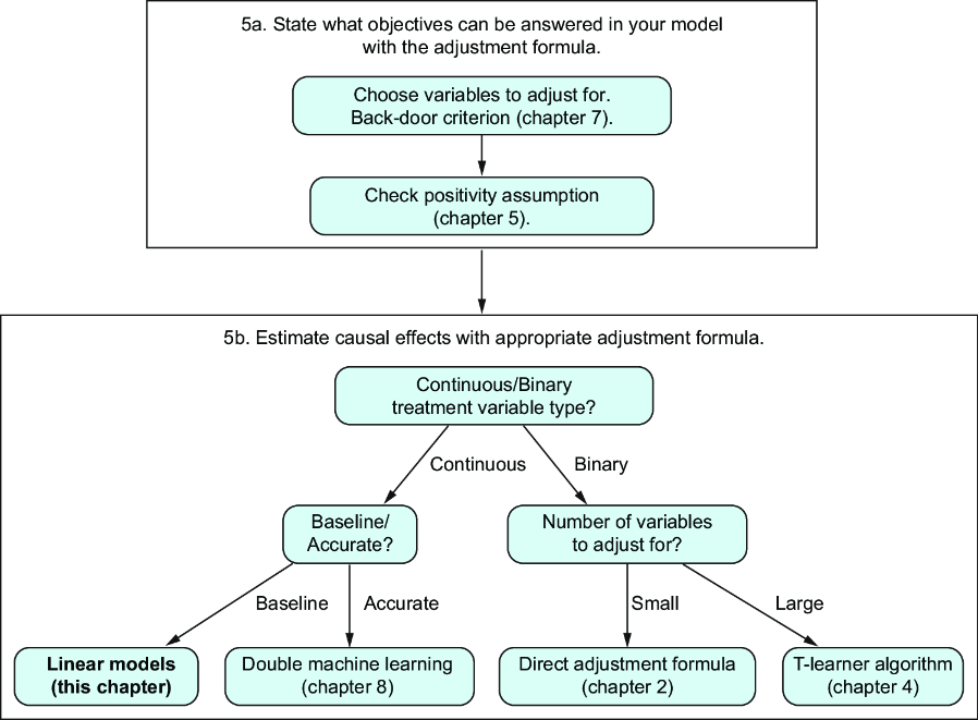
You are here
Apply the adjustment formula.
Although linear models are traditional, they remain widely used in many fields, including statistics, econometrics, and machine learning, demonstrating their enduring relevance and utility in both research and practical applications.