7 Dealing with complex graphs
This chapter covers
- A mathematical definition of a causal model
- Deriving conditional independencies between variables with d-separation
- Using the back-door criterion to decide which variables to put in the adjustment formula
We now know that one way to remove the effect of confounders is by using the adjustment formula. In real life, we work with complex DAGs, and we will have doubts about which variables to adjust for. Therefore, in this chapter, we answer the following question: given a particular DAG (simple or complex), a treatment, and outcome variables, which variables should we adjust for to estimate the average treatment effect (ATE)?
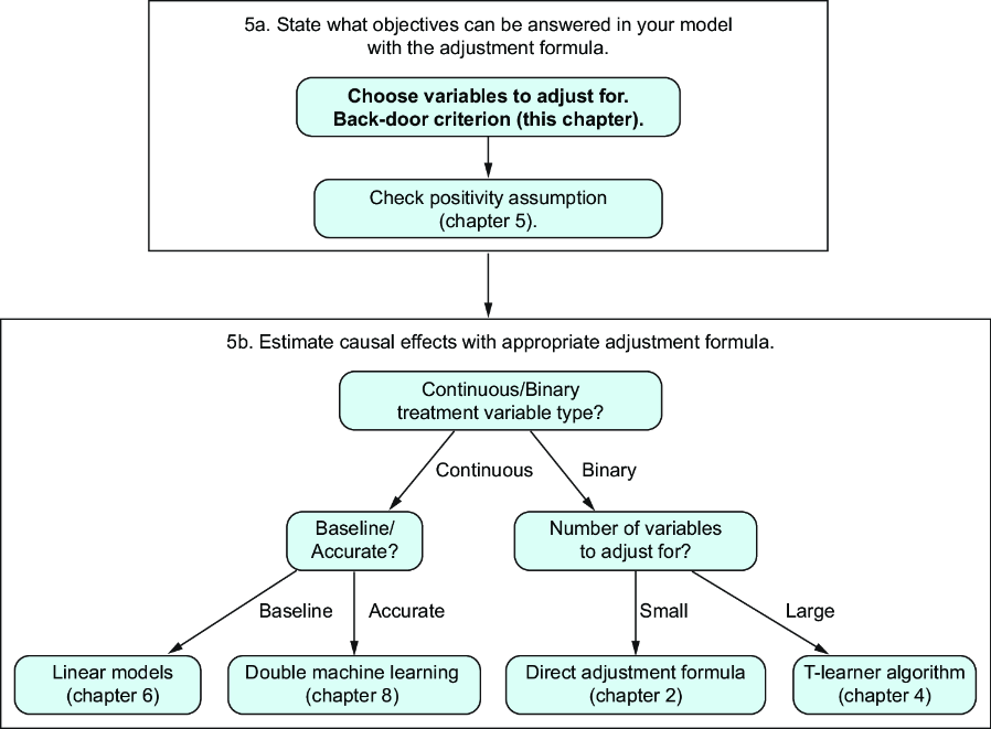
You are here
Applying the adjustment formula
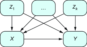
You may wonder why we didn’t have trouble choosing the right confounders in the previous chapters. We were working essentially with just one type of graph: the DAG in figure 7.1, where all confounders are known, observed, and without causal relations among them. So, to estimate the causal effect between X and Y, we need to adjust for confounders Z1, …, Zk. However, you will frequently find unobserved confounders with complex interactions in practice.
Figure 7.1 We want to estimate a causal effect between X and Y. In this graph, all confounders are known, so there is no problem with unobserved confounders.