9 Choosing the best forecasting KPI
In chapter 8, you learned how to compute various forecasting KPIs (Bias, MAE, MAPE, and RMSE—see table 9.1 for a recap). Unfortunately, as highlighted in the case study in section 9.4, depending on the KPI you pick, you might end up choosing different forecasts. (Remember, the objective of demand forecasting is to provide valuable information to the other teams in the supply chain so they can make appropriate decisions.)
Table 9.1 Forecasting Metrics (view table figure)
| Metric |
Formula |
|
|---|---|---|
| Bias |
|
=average(error) |
| MAE |
|
=average(|error|) |
| MAE% |
|
=sum(|error|)/sum(demand) |
| MAPE |
|
=average(|error|/demand) |
| RMSE |
|
=sqrt(average([forecast-demand]²)) |

In this chapter, we will further analyze these metrics’ pros and cons using two specific scenarios: extreme demand patterns (with outliers) and products with intermittent (sporadic) demand. Finally, we will conclude this chapter by selecting a combination of metrics that will provide a (very) good tradeoff between simplicity, accuracy, bias, and outlier sensitivity.
9.1 Extreme demand patterns
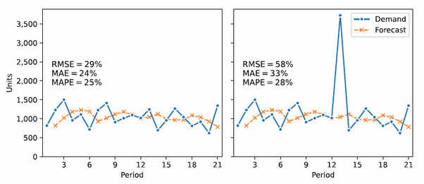
In the case of highly variable, sporadic demand (or the presence of outliers), RMSE might overreact to a few forecast errors as RMSE emphasizes the most significant errors (RMSE looks at squared errors). As you can see in figure 9.1, adding an outlier to a dataset will greatly impact RMSE.
Figure 9.1 Historical demand with and without outlier (Period 13)