Chapter 10. Analytics-on-read
This chapter covers
- Analytics-on-read versus analytics-on-write
- Amazon Redshift, a horizontally scalable columnar database
- Techniques for storing and widening events in Redshift
- Some example analytics-on-read queries
Up to this point, this book has largely focused on the operational mechanics of a unified log. When we have performed any analysis on our event streams, this has been primarily to put technology such as Apache Spark or Samza through its paces, or to highlight the various use cases for a unified log.
Part 3 of this book sees a change of focus: we will take an analysis-first look at the unified log, leading with the two main methodologies for unified log analytics and then applying various database and stream processing technologies to analyze our event streams.
What do we mean by unified log analytics? Simply put, unified log analytics is the examination of one or more of our unified log’s event streams to drive business value. It covers everything from detection of customer fraud, through KPI dashboards for busy executives, to predicting breakdowns of fleet vehicles or plant machinery. Often the consumer of this analysis will be a human or humans, but not necessarily: unified log analytics can just as easily drive an automated machine-to-machine response.
With unified log analytics having such a broad scope, we need a way of breaking down the topic further. A helpful distinction for analytics on event streams is between analytics-on-write versus analytics-on-read. The first section of this chapter will explain the distinction, and then we will dive into a complete case study of analytics-on-read. A new part of the book deserves a new figurative unified log owner, so for our case study we will introduce OOPS, a major package-delivery company.
Our case study will be built on top of the Amazon Redshift database. Redshift is a fully hosted (on Amazon Web Services) analytical database that uses columnar storage and speaks a variant of PostgreSQL. We will be using Redshift to try out a variety of analytics-on-read required by OOPS.
Let’s get started!
If we want to explore what is occurring in our event streams, where should we start? The Big Data ecosystem is awash with competing databases, batch- and stream-processing frameworks, visualization engines, and query languages. Which ones should we pick for our analyses?
The trick is to understand that all these myriad technologies simply help us to implement either analytics-on-write or analytics-on-read for our unified log. If we can understand these two approaches, the way we deliver our analytics by using these technologies should become much clearer.
Let’s imagine that we are in the BI team at OOPS, an international package-delivery company. OOPS has implemented a unified log using Amazon Kinesis that is receiving events emitted by OOPS delivery trucks and the handheld scanners of OOPS delivery drivers.
We know that as the BI team, we will be responsible for analyzing the OOPS event streams in all sorts of ways. We have some ideas of what reports to build, but these are just hunches until we are much more familiar with the events being generated by OOPS trucks and drivers out in the field. How can we get that familiarity with our event streams? This is where analytics-on-read comes in.
Analytics-on-read is really shorthand for a two-step process:
- Write all of our events to some kind of event store.
- Read the events from our event store to perform an analysis.
In other words: store first; ask questions later. Does this sound familiar? We’ve been here before, in chapter 7, where we archived all of our events to Amazon S3 and then wrote a simple Spark job to generate a simple analysis from those events. This was classic analytics-on-read: first we wrote our events to a storage target (S3), and only later did we perform the required analysis, when our Spark job read all of our events back from our S3 archive.
An analytics-on-read implementation has three key parts:
- A storage target to which the events will be written. We use the term storage target because it is more general than the term database.
- A schema, encoding, or format in which the events should be written to the storage target.
- A query engine or data processing framework to allow us to analyze the events as read from our storage target.
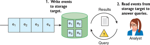
Figure 10.1 illustrates these three components.
Figure 10.1. For analytics-on-read, we first write events to our storage target in a predetermined format. Then when we have a query about our event stream, we run that query against our storage target and retrieve the results.
Storing data in a database so that it can be queried later is a familiar idea to almost all readers. And yet, in the context of the unified log, this is only half of the analytics story; the other half of the story is called analytics-on-write.
Let’s skip forward in time and imagine that we, the BI team at OOPS, have implemented some form of analytics-on-read on the events generated by our delivery trucks and drivers. The exact implementation of this analytics doesn’t particularly matter. For familiarity’s sake, let’s say that we again stored our events in Amazon S3 as JSON, and we then wrote a variety of Apache Spark jobs to derive insights from the event archive.
Regardless of the technology, the important thing is that as a team, we are now much more comfortable with the contents of our company’s unified log. And this familiarity has spread to other teams within OOPS, who are now making their own demands on our team:
- The executive team wants to see dashboards of key performance indicators (KPIs), based on the event stream and accurate to the last five minutes.
- The marketing team wants to add a parcel tracker on the website, using the event stream to show customers where their parcel is right now and when it’s likely to arrive.
- The fleet maintenance team wants to use simple algorithms (such as date of last oil change) to identify trucks that may be about to break down in mid-delivery.
Your first thought might be that our standard analytics-on-read could meet these use cases; it may well be that your colleagues have prototyped each of these requirements with a custom-written Spark job running on our archive of events in Amazon S3. But putting these three reports into production will take an analytical system with different priorities:
- Very low latency— The various dashboards and reports must be fed from the incoming event streams in as close to real time as possible. The reports must not lag more than five minutes behind the present moment.
- Supports thousands of simultaneous users— For example, the parcel tracker on the website will be used by large numbers of OOPS customers at the same time.
- Highly available— Employees and customers alike will be depending on these dashboards and reports, so they need to have excellent uptime in the face of server upgrades, corrupted events, and so on.
These requirements point to a much more operational analytical capability—one that is best served by analytics-on-write. Analytics-on-write is a four-step process:
- Read our events from our event stream.
- Analyze our events by using a stream processing framework.
- Write the summarized output of our analysis to a storage target.
- Serve the summarized output into real-time dashboards or reports.
We call this analytics-on-write because we are performing the analysis portion of our work prior to writing to our storage target; you can think of this as early, or eager, analysis, whereas analytics-on-read is late, or lazy, analysis. Again, this approach should seem familiar; when we were using Apache Samza in part 1, we were practicing a form of analytics-on-write!
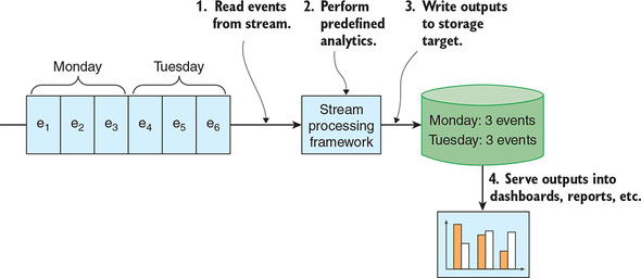
Figure 10.2 shows a simple example of analytics-on-write using a key-value store.
Figure 10.2. With analytics-on-write, the analytics are performed in stream, typically in close to real time, and the outputs of the analytics are written to the storage target. Those outputs can then be served into dashboards and reports.
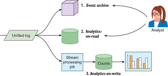
As the OOPS BI team, how should we choose between analytics-on-read and analytics-on-write? Strictly speaking, we don’t have to choose, as illustrated in figure 10.3. We can attach multiple analytics applications, both read and write, to process the event streams within OOPS’s unified log.
Figure 10.3. Our unified log feeds three discrete systems: our event archive, an analytics-on-read system, and an analytics-on-write system. Event archives were discussed in chapter 7.
Most organizations, however, will start with analytics-on-read. Analytics-on-read lets you explore your event data in a flexible way: because you have all of your events stored and a query language to interrogate them, you can answer pretty much any question asked of you. Specific analytics-on-write requirements will likely come later, as this initial analytical understanding percolates through your business.
In chapter 11, we will explore analytics-on-write in more detail, which should give you a better sense of when to use it; in the meantime, table 10.1 sets out some of the key differences between the two approaches.
Table 10.1. Comparing the main attributes of analytics-on-read to analytics-on-write (view table figure)
| Analytics-on-write |
|
|---|---|
| Predetermined storage format | Predetermined storage format |
| Flexible queries | Predetermined queries |
| High latency | Low latency |
| Support 10–100 users | Support 10,000s of users |
| Simple (for example, HDFS) or sophisticated (for example, HP Vertica) storage target | Simple storage target (for example, key-value store) |
| Sophisticated query engine or batch processing framework | Simple (for example, AWS Lambda) or sophisticated (for example, Apache Samza) stream processing framework |
It’s our first day on the OOPS BI team, and we have been asked to familiarize ourselves with the various event types being generated by OOPS delivery trucks and drivers. Let’s get started.
We quickly learn that three types of events are related to the delivery trucks themselves:
- Delivery truck departs from location at time
- Delivery truck arrives at location at time
- Mechanic changes oil in delivery truck at time
We ask our new colleagues about the three entities involved in our events: delivery trucks, locations, and employees. They talk us through the various properties that are stored against each of these entities when the event is emitted by the truck. Figure 10.4 illustrates these properties.
Figure 10.4. The three entities represented in our delivery-truck events are the delivery truck itself, a location, and an employee. All three of these entities have minimal properties—just enough to uniquely identify the entity.
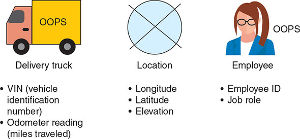
Note how few properties there are in these three event entities. What if we want to know more about a specific delivery truck or the employee changing its oil? Our colleagues in BI assure us that this is possible: they have access to the OOPS vehicle database and HR systems, containing data stored against the vehicle identification number (VIN) and the employee ID. Hopefully, we can use this additional data later.
Now we turn to the delivery drivers themselves. According to our BI team, just two events matter here:
- Driver delivers package to customer at location at time
- Driver cannot find customer for package at location at time
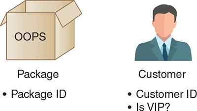
In addition to employees and locations, which we are familiar with, these events involve two new entity types: packages and customers. Again, our BI colleagues talk us through the properties attached to these two entities in the OOPS event stream. As you can see in figure 10.5, these entities have few properties—just enough data to uniquely identify the package or customer.
Figure 10.5. The events generated by our delivery drivers involve two additional entities: packages and customers. Again, both entities have minimal properties in the OOPS event model.
The event model used by OOPS is slightly different from the one we used in parts 1 and 2 of the book. Each OOPS event is expressed in JSON and has the following properties:
- A short tag describing the event (for example, TRUCK_DEPARTS or DRIVER_MISSES_CUSTOMER)
- A timestamp at which the event took place
- Specific slots related to each of the entities that are involved in this event
Here is an example of a Delivery truck departs from location at time event:
{ "event": "TRUCK_DEPARTS", "timestamp": "2018-11-29T14:48:35Z",
 "vehicle": { "vin": "1HGCM82633A004352", "mileage": 67065 }, "location":
 { "longitude": 39.9217860, "latitude": -83.3899969, "elevation": 987 } }
The BI team at OOPS has made sure to document the structure of all five of their event types by using JSON Schema; remember that we introduced JSON Schema in chapter 6. In the following listing, you can see the JSON schema file for the Delivery truck departs event.
Listing 10.1. truck_departs.json
{
  "type": "object",
  "properties": {
    "event": {
      "enum": [ "TRUCK_DEPARTS" ]
    },
    "timestamp": {
      "type": "string",
      "format": "date-time"
    },
    "vehicle": {
      "type": "object",
      "properties": {
        "vin": {
          "type": "string",
          "minLength": 17,
          "maxLength": 17
        },
        "mileage": {
          "type": "integer",
          "minimum": 0,
          "maximum": 2147483647
        }
      },
      "required": [ "vin", "mileage" ],
      "additionalProperties": false
    },
    "location": {
      "type": "object",
      "properties": {
        "latitude": {
          "type": "number"
        },
        "longitude": {
          "type": "number"
        },
        "elevation": {
          "type": "integer",
          "minimum": -32768,
          "maximum": 32767
        }
      },
      "required": [ "longitude", "latitude", "elevation" ],
      "additionalProperties": false
    }
  },
  "required": [ "event", "timestamp", "vehicle", "location" ],
  "additionalProperties": false
}
By the time we join the BI team, the unified log has been running at OOPS for several months. The BI team has implemented a process to archive the events being generated by the OOPS delivery trucks and drivers. This archival approach is similar to that taken in chapter 7:
- Our delivery trucks and our drivers’ handheld computers emit events that are received by an event collector (most likely a simple web server).
- The event collector writes these events to an event stream in Amazon Kinesis.
- A stream processing job reads the stream of raw events and validates the events against their JSON schemas.
- Events that fail validation are written to a second Kinesis stream, called the bad stream, for further investigation.
- Events that pass validation are written to an Amazon S3 bucket, and partitioned into folders based on the event type.
Phew—there is a lot to take in here, and you may be thinking that these steps are not relevant to us, because they take place upstream of our analytics. But a good analyst or data scientist will always take the time to understand the source-to-sink lineage of their event stream. We should be no different! Figure 10.6 illustrates this five-step event-archiving process.
Figure 10.6. Events flow from our delivery trucks and drivers into an event collector. The event collector writes the events into a raw event stream in Kinesis. A stream processing job reads this stream, validates the events, and archives the valid events to Amazon S3; invalid events are written to a second stream.
;%22/%3E%3C/svg%3E)
A few things to note before we continue:
- The validation step is important, because it ensures that the archive of events in Amazon S3 consists only of well-formed JSON files that conform to JSON Schema.
- In this chapter, we won’t concern ourselves further with the bad stream, but see chapter 8 for a more thorough exploration of happy versus failure paths.
- The events are stored in Amazon S3 in uncompressed plain-text files, with each event’s JSON separated by a newline. This is called newline-delimited JSON (http://ndjson.org).
To check the format of the events ourselves, we can download them from Amazon S3:
$ aws s3 cp s3://ulp-assets-2019/ch10/data/ . --recursive --profile=ulp
download: s3://ulp-assets-2019/ch10/data/events.ndjson to ./events.ndjson
$ head -3 events.ndjson
{"event":"TRUCK_DEPARTS", "location":{"elevation":7, "latitude":51.522834,
 "longitude": -0.081813}, "timestamp":"2018-11-01T01:21:00Z", "vehicle":
 {"mileage":32342, "vin":"1HGCM82633A004352"}}
{"event":"TRUCK_ARRIVES", "location":{"elevation":4, "latitude":51.486504,
 "longitude": -0.0639602}, "timestamp":"2018-11-01T05:35:00Z", "vehicle":
 {"mileage":32372, "vin":"1HGCM82633A004352"}}
{"employee":{"id":"f6381390-32be-44d5-9f9b-e05ba810c1b7", "jobRole":
 "JNR_MECHANIC"}, "event":"MECHANIC_CHANGES_OIL", "timestamp":
 "2018-11-01T08:34:00Z", "vehicle": {"mileage":32372, "vin":
 "1HGCM82633A004352"}}
We can see some events that seem to relate to a trip to the garage to change a delivery truck’s oil. And it looks like the events conform to the JSON schema files written by our colleagues, so we’re ready to move onto Redshift.
Our colleagues in BI have selected Amazon Redshift as the storage target for our analytics-on-read endeavors. In this section, we will help you become familiar with Redshift before designing an event model to store our various event types in the database.
Amazon Redshift is a column-oriented database from Amazon Web Services that has grown increasingly popular for event analytics. Redshift is a fully hosted database, available exclusively on AWS and built using columnar database technology from ParAccel (now part of Actian). ParAccel’s technology is based on PostgreSQL, and you can largely use PostgreSQL-compatible tools and drivers to connect to Redshift.
Redshift has evolved significantly since its launch in early 2013, and now sports distinct features of its own; even if you are familiar with PostgreSQL or ParAccel, we recommend checking out the official Redshift documentation from AWS at https://docs.aws.amazon.com/redshift/.
Redshift is a massively parallel processing (MPP) database technology that allows you to scale horizontally by adding additional nodes to your cluster as your event volumes grow. Each Redshift cluster has a leader node and at least one compute node. The leader node is responsible for receiving SQL queries from a client, creating a query execution plan, and then farming out that query plan to the compute nodes. The compute nodes execute the query execution plan and then return their portion of the results back to the leader node. The leader node then consolidates the results from all of the compute nodes and returns the final results to the client. Figure 10.7 illustrates this data flow.
Figure 10.7. A Redshift cluster consists of a leader node and at least one compute node. Queries flow from a client application through the leader node to the compute nodes; the leader node is then responsible for consolidating the results and returning them to the client.
;%22/%3E%3C/svg%3E)
Redshift has attributes that make it a great fit for many analytics-on-read workloads. Its killer feature is the ability to run PostgreSQL-flavored SQL, including full inter-table JOINs and windowing functions, over many billions of events. But it’s worth understanding the design decisions that have gone into Redshift, and how those decisions enable some things while making other things more difficult. Table 10.2 sets out these related strengths and weaknesses of Redshift.
Table 10.2. Strengths and weaknesses of Amazon Redshift (view table figure)
In any case, our BI colleagues at OOPS have asked us to set up a new Redshift cluster for some analytics-on-write experiments, so let’s get started!
Our colleagues haven’t given us access to the OOPS AWS account yet, so we will have to create the Redshift cluster in our own AWS account. Let’s do some research and select the smallest and cheapest Redshift cluster available; we must remember to shut it down as soon as we are finished with it as well.
At the time of writing, four Amazon Elastic Compute Cloud (EC2) instance types are available for a Redshift cluster, as laid out in table 10.3.[1]
1In table 10.3, the “Instance type” column uses “dc” and “ds” prefixes to refer to dense compute and dense storage, respectively. In the “CPU” column, “CUs” refers to compute units.
A cluster must consist exclusively of one instance type; you cannot mix and match. Some instance types allow for single-instance clusters, whereas other instance types require at least two instances. Confusingly, AWS refers to this as single-node versus multi-node—confusing because a single-node cluster still has a leader node and a compute node, but they simply reside on the same EC2 instance. On a multi-node cluster, the leader node is separate from the compute nodes.
Table 10.3. Four EC2 instance types available for a Redshift cluster (view table figure)
| Instance type |
Storage |
CPU |
Memory |
Single-instance okay? |
|---|---|---|---|---|
| dc2.large | 160 GB SSD | 7 EC2 CUs | 15 GiB | Yes |
| dc2.8xlarge | 2.56 TB SSD | 99 EC2 CUs | 244 GiB | No |
| ds2.xlarge | 2 TB HDD | 14 EC2 CUs | 31 GiB | Yes |
| ds2.8xlarge | 16 TB HDD | 116 EC2 CUs | 244 GiB | No |
Currently, you can try Amazon Redshift for two months for free (provided you’ve never created an Amazon Redshift cluster before) and you get a cluster consisting of a single dc2.large instance, so that’s what we will set up using the AWS CLI. Assuming you are working in the book’s Vagrant virtual machine and still have your ulp profile set up, you can simply type this:
$ aws redshift create-cluster --cluster-identifier ulp-ch10 \
--node-type  dc2.large --db-name ulp --master-username ulp \
--master-user-password Unif1edLP --cluster-type single-node \
--region us-east-1 --profile ulp
As you can see, creating a new cluster is simple. In addition to specifying the cluster type, we create a master username and password, and create an initial database called ulp. Press Enter, and the AWS CLI should return JSON of the new cluster’s details:
{
    "Cluster": {
        "ClusterVersion": "1.0",
        "NumberOfNodes": 1,
        "VpcId": "vpc-3064fb55",
        "NodeType": "dc1.large",
        ...
    }
}
Let’s log in to the AWS UI and check out our Redshift cluster:
- On the AWS dashboard, check that the AWS region in the header at the top right is set to N. Virginia (it is important to select that region for reasons that will become clear in section 10.3).
- Click Redshift in the Database section.
- Click the listed cluster, ulp-ch10.
After a few minutes, the status should change from Creating to Available. The details for your cluster should look similar to those shown in figure 10.8.
Figure 10.8. The Configuration tab of the Redshift cluster UI provides all the available metadata for our new cluster, including status information and helpful JDBC and ODBC connection URIs.
;%22/%3E%3C/svg%3E)
Our database is alive! But before we can connect to it, we will have to whitelist our current public IP address for access. To do this, we first need to create a security group:
$ aws ec2 create-security-group --group-name redshift \
--description
{
    "GroupId": "sg-5b81453c"
}
Now let’s authorize our IP address, making sure to update the group_id with your own value from the JSON returned by the preceding command:
$ group_id=sg-5b81453c
$ public_ip=$(dig +short myip.opendns.com @resolver1.opendns.com)
$ aws ec2 authorize-security-group-ingress --group-id ${group_id} \
--port 5439 --cidr ${public_ip}/32 --protocol tcp --region us-east-1 \
--profile ulp
Now we update our cluster to use this security group, again making sure to update the group ID:
$ aws redshift modify-cluster --cluster-identifier ulp-ch10 \

{
    "Cluster": {
        "PubliclyAccessible": true,
        "MasterUsername": "ulp",
        "VpcSecurityGroups": [
            {
                "Status": "adding",
                "VpcSecurityGroupId": "sg-5b81453c"
            }
        ],
        ...
The returned JSON helpfully shows us the newly added security group near the top. Phew! Now we are ready to connect to our Redshift cluster and check that we can execute SQL queries. We are going to use a standard PostgreSQL client to access our Redshift cluster. If you are working in the book’s Vagrant virtual machine, you will find the command-line tool psql installed and ready to use. If you have a preferred PostgreSQL GUI, that should work fine too.
First let’s check that we can connect to the cluster. Update the first line shown here to point to the Endpoint URI, as shown in the Configuration tab of the Redshift cluster UI:
$ host=ulp-ch10.ccxvdpz01xnr.us-east-1.redshift.amazonaws.com
$ export PGPASSWORD=Unif1edLP
$ psql ulp --host ${host} --port 5439 --username ulp
psql (8.4.22, server 8.0.2)
WARNING: psql version 8.4, server version 8.0.
         Some psql features might not work.
SSL connection (cipher: ECDHE-RSA-AES256-SHA, bits: 256)
Type "help" for help.

ulp=#
Success! Let’s try a simple SQL query to show the first three tables in our database:
ulp=# SELECT DISTINCT tablename FROM pg_table_def LIMIT 3;
        tablename
--------------------------
 padb_config_harvest
 pg_aggregate
 pg_aggregate_fnoid_index
(3 rows)
Our Redshift cluster is up and running, accessible from our computer’s IP address and responding to our SQL queries. We’re now ready to start designing the OOPS event warehouse to support our analytics-on-read requirements.
Remember that at OOPS we have five event types, each tracking a distinct action involving a subset of the five business entities that matter at OOPS: delivery trucks, locations, employees, packages, and customers. We need to store these five event types in a table structure in Amazon Redshift, with maximal flexibility for whatever analytics-on-read we may want to perform in the future.
How should we store these events in Redshift? One naïve approach would be to define a table in Redshift for each of our five event types. This approach, depicted in figure 10.9, has one obvious issue: to perform any kind of analysis across all event types, we have to use the SQL UNION command to join five SELECTs together. Imagine if we had 30 or 300 event types—even simple counts of events per hour would become extremely painful!
Figure 10.9. Following the table-per-event approach, we would create five tables for OOPS. Notice how the entities recorded in the OOPS events end up duplicated multiple times across the various event types.
;%22/%3E%3C/svg%3E)
This table-per-event approach has a second issue: our five business entities are duplicated across multiple event tables. For example, the columns for our employee are duplicated in three tables; the columns for a geographical location are in four of our five tables. This is problematic for a few reasons:
- If OOPS decides, say, that all locations should also have a zip code, then we have to upgrade four tables to add the new column.
- If we have a table of employee details in Redshift and we want to JOIN it to the employee ID, we have to write separate JOINs for three separate event tables.
- If we want to analyze a type of entity rather than a type of event (for example, “which locations saw the most event activity on Tuesday?”), then the data we care about is scattered over multiple tables.
If a table per event type doesn’t work, what are the alternatives? Broadly, we have two options: a fat table or shredded entities.
- A short tag describing the event (or example, TRUCK_DEPARTS or DRIVER_MISSES_CUSTOMER)
- A timestamp at which the event took place
- Columns for each of the entities involved in our events
The table is sparsely populated, meaning that columns will be empty if an event does not feature a given entity. Figure 10.10 depicts this approach.
Figure 10.10. The fat-table approach records all event types in a single table, which has columns for each entity involved in the event. We refer to this table as “sparsely populated” because entity columns will be empty if a given event did not record that entity.
;%22/%3E%3C/svg%3E)
For a simple event model like OOPS’s, the fat table can work well: it is straightforward to define, easy to query, and relatively straightforward to maintain. But it starts to show its limits as we try to model more sophisticated events; for example:
- What if we want to start tracking events between two employees (for example, a truck handover)? Do we have to add another set of employee columns to the table?
- How do we support events involving a set of the same entity—for example, when an employee packs n items into a package?
Even so, you can go a long way with a fat table of your events in a database such as Redshift. Its simplicity makes it quick to get started and lets you focus on analytics rather than time-consuming schema design. We used the fat-table approach exclusively at Snowplow for about two years before starting to implement another option, described next.
Through trial and error, we evolved a third approach at Snowplow, which we refer to as shredded entities. We still have a master table of events, but this time it is “thin,” containing only the following:
- A short tag describing the event (for example, TRUCK_DEPARTS)
- A timestamp at which the event took place
- An event ID that uniquely identifies the event (UUID4s work well)
Accompanying this master table, we also now have a table per entity; so in the case of OOPS, we would have five additional tables—one each for delivery trucks, locations, employees, packages, and customers. Each entity table contains all the properties for the given entity, but crucially it also includes a column with the event ID of the parent event that this entity belongs to. This relationship allows an analyst to JOIN the relevant entities back to their parent events. Figure 10.11 depicts this approach.
Figure 10.11. In the shredded-entities approach, we have a “thin” master events table that connects via an event ID to dedicated entity-specific tables. The name comes from the idea that the event has been “shredded” into multiple tables.
;%22/%3E%3C/svg%3E)
- We can support events that consist of multiple instances of the same entity, such as two employees or n items in a package.
- Analyzing entities is super simple: all of the data about a single entity type is available in a single table.
- If our definition of an entity changes (for example, we add a zip code to a location), we have to update only the entity-specific table, not the main table.
Although it is undoubtedly powerful, implementing the shredded-entities approach is complex (and is, in fact, an ongoing project at Snowplow). Our colleagues at OOPS don’t have that kind of patience, so for this chapter we are going to design, load, and analyze a fat table instead. Let’s get started.
We already know the design of our fat events table; it is set out in figure 10.10. To deploy this as a table into Amazon Redshift, we will write SQL-flavored data-definition language (DDL); specifically, we need to craft a CREATE TABLE statement for our fat events table.
Writing table definitions by hand is a tedious exercise, especially given that our colleagues at OOPS have already done the work of writing JSON schema files for all five of our event types! Luckily, there is another way: at Snowplow we have open sourced a CLI tool called Schema Guru that can, among other things, autogenerate Redshift table definitions from JSON Schema files. Let’s start by downloading the five events’ JSON Schema files from the book’s GitHub repository:
$ git clone https://github.com/alexanderdean/Unified-Log-Processing.git
$ cd Unified-Log-Processing/ch10/10.2 && ls schemas
driver_delivers_package.json  mechanic_changes_oil.json  truck_departs.json
driver_misses_customer.json   truck_arrives.json
Now let’s install Schema Guru:
$ ZIPFILE=schema_guru_0.6.2.zip
$ cd .. && wget http://dl.bintray.com/snowplow/snowplow-generic/${ZIPFILE}
$ unzip ${ZIPFILE}
We can now use Schema Guru in generate DDL mode against our schemas folder:
$ ./schema-guru-0.6.2 ddl –raw-mode ./schemas
File [Unified-Log-Processing/ch10/10.2/./sql/./driver_delivers_package.sql]
 was written successfully!
File [Unified-Log-Processing/ch10/10.2/./sql/./driver_misses_customer.sql]
 was written successfully!
File [Unified-Log-Processing/ch10/10.2/./sql/./mechanic_changes_oil.sql]
 was written successfully!
File [Unified-Log-Processing/ch10/10.2/./sql/./truck_arrives.sql]
 was written successfully!
File [Unified-Log-Processing/ch10/10.2/./sql/./truck_departs.sql]
 was written successfully!
After you have run the preceding command, you should have a definition for our fat events table identical to the one in the following listing.
Listing 10.2. events.sql
CREATE TABLE IF NOT EXISTS events (
    "event"              VARCHAR(23) NOT NULL,
    "timestamp"          TIMESTAMP   NOT NULL,
    "customer.id"        CHAR(36),
    "customer.is_vip"    BOOLEAN,
    "employee.id"        CHAR(36),
    "employee.job_role"  VARCHAR(12),
    "location.elevation" SMALLINT,
    "location.latitude"  DOUBLE PRECISION,
    "location.longitude" DOUBLE PRECISION,
    "package.id"         CHAR(36),
    "vehicle.mileage"    INT,
    "vehicle.vin"        CHAR(17)
);
To save you the typing, the events table is already available in the book’s GitHub repository. We can deploy it into our Redshift cluster like so:
ulp=# \i /vagrant/ch10/10.2/sql/events.sql
CREATE TABLE
We now have our fat events table in Redshift.
Our fat events table is now sitting empty in Amazon Redshift, waiting to be populated with our archive of OOPS events. In this section, we will walk through a simple manual process for loading the OOPS events into our table.
These kinds of processes are often referred to as ETL, an old data warehousing acronym for extract, transform, load. As MPP databases such as Redshift have grown more popular, the acronym ELT has also emerged, meaning that the data is loaded into the database before further transformation is applied.
If you have previously worked with databases such as PostgreSQL, SQL Server, or Oracle, you are probably familiar with the COPY statement that loads one or more comma- or tab-separated files into a given table in the database. Figure 10.12 illustrates this approach.
Figure 10.12. A Redshift COPY statement lets you load one or more comma- or tab-separated flat files into a table in Redshift. The “columns” in the flat files must contain data types that are compatible with the table’s corresponding columns.
;%22/%3E%3C/svg%3E)
In addition to a regular COPY statement, Amazon Redshift supports something rather more unique: a COPY from JSON statement, which lets us load files of newline-delimited JSON data into a given table.[2] This load process depends on a special file, called a JSON Paths file, which provides a mapping from the JSON structure to the table. The format of the JSON Paths file is ingenious. It’s a simple JSON array of strings, and each string is a JSON Path expression identifying which JSON property to load into the corresponding column in the table. Figure 10.13 illustrates this process.
2The following article describes how to load JSON files into a Redshift table: https://docs.aws.amazon.com/redshift/latest/dg/copy-usage_notes-copy-from-json.html
Figure 10.13. The COPY from JSON statement lets us use a JSON Paths configuration file to load files of newline-separated JSON data into a Redshift table. The array in the JSON Paths file should have an entry for each column in the Redshift table.
;%22/%3E%3C/svg%3E)
If it’s helpful, you can imagine that the COPY from JSON statement first creates a temporary CSV or TSV flat file from the JSON data, and then those flat files are COPY’ed into the table.
In this chapter, we want to create a simple process for loading the OOPS events into Redshift from JSON with as few moving parts as possible. Certainly, we don’t want to have to write any (non-SQL) code if we can avoid it. Happily, Redshift’s COPY from JSON statement should let us load our OOPS event archive directly into our fat events table. A further stroke of luck: we can use a single JSON Paths file to load all five of our event types! This is because OOPS’s five event types have a predictable and shared structure (the five entities again), and because a COPY from JSON can tolerate specified JSON Paths not being found in a given JSON (it will simply set those columns to null).
We are now ready to write our JSON Paths file. Although Schema Guru can generate these files automatically, it’s relatively simple to do this manually: we just need to use the correct syntax for the JSON Paths and ensure that we have an entry in the array for each column in our fat events table. The following listing contains our populated JSON Paths file.
Listing 10.3. events.jsonpaths
{
  "jsonpaths": [
    "$.event",             #1
    "$.timestamp",         #1
    "$.customer.id",       #2
    "$.customer.isVip",
    "$.employee.id",
    "$.employee.jobRole",
    "$.location.elevation",
    "$.location.latitude",
    "$.location.longitude",
    "$.package.id",
    "$.vehicle.mileage",
    "$.vehicle.vin"
  ]
}
A Redshift COPY from JSON statement requires the JSON Paths file to be available on Amazon S3, so we have uploaded the events.jsonpaths file to Amazon S3 at the following path:
s3://ulp-assets-2019/ch10/jsonpaths/event.jsonpaths
We are now ready to load all of the OOPS event archive into Redshift! We will do this as a one-time action, although you could imagine that if our analytics-on-read are fruitful, our OOPS colleagues could configure this load process to occur regularly—perhaps nightly or hourly. Reopen your psql connection if it has closed:
$ psql ulp --host ${host} --port 5439 --username ulp
...
ulp=#
Now execute your COPY from JSON statement, making sure to update your AWS access key ID and secret access key (the XXXs) accordingly:
ulp=# COPY events FROM 's3://ulp-assets-2019/ch10/jsonpaths/data/' \
 CREDENTIALS 'aws_access_key_id=XXX;aws_secret_access_key=XXX' JSON \
's3://ulp-assets-2019/ch10/jsonpaths/event.jsonpaths' \
REGION 'us-east-1' TIMEFORMAT 'auto';
INFO:  Load into table 'events' completed, 140 record(s) loaded successfully.
COPY
- The AWS CREDENTIALS will be used to access the data in S3 and the JSON Paths file.
- The REGION parameter specifies the region in which the data and JSON Paths file are located. If you get an error similar to S3ServiceException: The bucket you are attempting to access must be addressed using the specified endpoint, it means that your Redshift cluster and your S3 bucket are in different regions. Both must be in the same region for the COPY command to succeed.
- TIMEFORMAT 'auto' allows the COPY command to autodetect the timestamp format used for a given input field.
Let’s perform a simple query now to get an overview of the events we have loaded:
ulp=# SELECT event, COUNT(*) FROM events GROUP BY 1 ORDER BY 2 desc;
          event          | count
-------------------------+-------
 TRUCK_DEPARTS           |    52
 TRUCK_ARRIVES           |    52
 MECHANIC_CHANGES_OIL    |    19
 DRIVER_DELIVERS_PACKAGE |     5
 DRIVER_MISSES_CUSTOMER  |     2
(5 rows)
Great—we have loaded some OOPS delivery events into Redshift!
We now have our event archive loaded into Redshift—our OOPS teammates will be pleased! But let’s take a look at an individual event:
\x on
Expanded display is on.
ulp=# SELECT * FROM events WHERE event='DRIVER_MISSES_CUSTOMER' LIMIT 1;
-[ RECORD 1 ]------+-------------------------------------
event              | DRIVER_MISSES_CUSTOMER
timestamp          | 2018-11-11 12:27:00
customer.id        | 4594f1a1-a7a2-4718-bfca-6e51e73cc3e7
customer.is_vip    | f
employee.id        | 54997a47-252d-499f-a54e-1522ac49fa48
employee.job_role  | JNR_DRIVER
location.elevation | 102
location.latitude  | 51.4972997
location.longitude | -0.0955459
package.id         | 14a714cf-5a89-417e-9c00-f2dba0d1844d
vehicle.mileage    |
vehicle.vin        |
Doesn’t it look a bit, well, uninformative? The event certainly has lots of identifiers, but few interesting data points: a VIN uniquely identifies an OOP delivery truck, but it doesn’t tell us how old the truck is, or the truck’s make or model. It would be ideal to look up these entity identifiers in a reference database, and then add this extra entity data to our events. In analytics speak, this is called dimension widening, because we are taking one of the dimensions in our event data and widening it with additional data points.
Imagine that we ask our colleagues about this, and one of them shares with us a Redshift-compatible SQL file of OOPS reference data. The SQL file creates and populates four tables covering same of the entities involved in our events: vehicles, employees, customers, and packages. OOPS has no reference data for locations, but no matter. Longitude, latitude, and elevation give us ample information about each location. Each of the four entity tables contains an ID that can be used to join a given row with a corresponding entity in our events table. Figure 10.14 illustrates these relationships.
Figure 10.14. We can use the entity identifiers in our fat-events table to join our event back to per-entity reference tables. This dimension widening gives us much richer events to analyze.
;%22/%3E%3C/svg%3E)
The SQL file for our four reference tables and their rows is shown in listing 10.4. This is deliberately a hugely abbreviated reference dataset. In reality, a company such as OOPS would have significant volumes of reference data, and synchronizing that data into the event warehouse to support analytics-on-read would be a significant and ongoing ETL project itself.
Listing 10.4. reference.sql
CREATE TABLE vehicles(
  vin CHAR(17) NOT NULL,
  make VARCHAR(32) NOT NULL,
  model VARCHAR(32) NOT NULL,
  year SMALLINT);
INSERT INTO vehicles VALUES
  ('1HGCM82633A004352', 'Ford', 'Transit', 2005),
  ('JH4TB2H26CC000000', 'VW', 'Caddy', 2010),
  ('19UYA31581L000000', 'GMC', 'Savana', 2011);

CREATE TABLE employees(
  id CHAR(36) NOT NULL,
  name VARCHAR(32) NOT NULL,
  dob DATE NOT NULL);
INSERT INTO employees VALUES
  ('f2caa6a0-2ce8-49d6-b793-b987f13cfad9', 'Amanda', '1992-01-08'),
  ('f6381390-32be-44d5-9f9b-e05ba810c1b7', 'Rohan', '1983-05-17'),
  ('3b99f162-6a36-49a4-ba2a-375e8a170928', 'Louise', '1978-11-25'),
  ('54997a47-252d-499f-a54e-1522ac49fa48', 'Carlos', '1985-10-27'),
  ('c4b843f2-0ef6-4666-8f8d-91ac2e366571', 'Andreas', '1994-03-13');

CREATE TABLE packages(
  id CHAR(36) NOT NULL,
  weight INT NOT NULL);
INSERT INTO packages VALUES
  ('c09e4ee4-52a7-4cdb-bfbf-6025b60a9144', 564),
  ('ec99793d-94e7-455f-8787-1f8ebd76ef61', 1300),
  ('14a714cf-5a89-417e-9c00-f2dba0d1844d', 894),
  ('834bc3e0-595f-4a6f-a827-5580f3d346f7', 3200),
  ('79fee326-aaeb-4cc6-aa4f-f2f98f443271', 2367);

CREATE TABLE customers(
  id CHAR(36) NOT NULL,
  name VARCHAR(32) NOT NULL,
  zip_code VARCHAR(10) NOT NULL);
INSERT INTO customers VALUES
  ('b39a2b30-049b-436a-a45d-46d290df65d3', 'Karl', '99501'),
  ('4594f1a1-a7a2-4718-bfca-6e51e73cc3e7', 'Maria', '72217-2517'),
  ('b1e5d874-963b-4992-a232-4679438261ab', 'Amit', '90089');
To save you the typing, this reference data is again available in the book’s GitHub repository. You can run it against your Redshift cluster like so:
ulp=# \i /vagrant/ch10/10.4/sql/reference.sql
CREATE TABLE
INSERT 0 3
CREATE TABLE
INSERT 0 5
CREATE TABLE
INSERT 0 5
CREATE TABLE
INSERT 0 3
Let’s get a feel for the reference data with a simple LEFT JOIN of the vehicles table back onto the events table:
ulp=# SELECT e.event, e.timestamp, e."vehicle.vin", v.* FROM events e \
 LEFT JOIN vehicles v ON e."vehicle.vin" = v.vin LIMIT 1;
-[ RECORD 1 ]--------------------
event       | TRUCK_ARRIVES
timestamp   | 2018-11-01 03:37:00
vehicle.vin | 1HGCM82633A004352
vin         | 1HGCM82633A004352
make        | Ford
model       | Transit
year        | 2005
The event types that involve a vehicle entity will have all of the fields from the vehicles table (v.*) populated. This is a good start, but we don’t want to have to manually construct these JOINs for every query. Instead, let’s create a single Redshift view that joins all of our reference tables back to the fat events table, to create an even fatter table. This view is shown in the following listing.
Listing 10.5. widened.sql
CREATE VIEW widened AS
  SELECT
    ev."event"              AS "event",
    ev."timestamp"          AS "timestamp",
    ev."customer.id"        AS "customer.id",
    ev."customer.is_vip"    AS "customer.is_vip",
    c."name"                AS "customer.name",
    c."zip_code"            AS "customer.zip_code",
    ev."employee.id"        AS "employee.id",
    ev."employee.job_role"  AS "employee.job_role",
    e."name"                AS "employee.name",
    e."dob"                 AS "employee.dob",
    ev."location.latitude"  AS "location.latitude",
    ev."location.longitude" AS "location.longitude",
    ev."location.elevation" AS "location.elevation",
    ev."package.id"         AS "package.id",
    p."weight"              AS "package.weight",
    ev."vehicle.vin"        AS "vehicle.vin",
    ev."vehicle.mileage"    AS "vehicle.mileage",
    v."make"                AS "vehicle.make",
    v."model"               AS "vehicle.model",
    v."year"                AS "vehicle.year"
  FROM events ev
    LEFT JOIN vehicles v  ON ev."vehicle.vin" = v.vin
    LEFT JOIN employees e ON ev."employee.id" = e.id
    LEFT JOIN packages p  ON ev."package.id"  = p.id
    LEFT JOIN customers c ON ev."customer.id" = c.id;
Again, this is available from the GitHub repository, so you can run it against your Redshift cluster like so:
ulp=# \i /vagrant/ch10/10.4/sql/widened.sql
CREATE VIEW
Let’s now get an event back from the view:
ulp=# SELECT * FROM widened WHERE event='DRIVER_MISSES_CUSTOMER' LIMIT 1;
-[ RECORD 1 ]------+-------------------------------------
event              | DRIVER_MISSES_CUSTOMER
timestamp          | 2018-11-11 12:27:00
customer.id        | 4594f1a1-a7a2-4718-bfca-6e51e73cc3e7
customer.is_vip    | f
customer.name      | Maria
customer.zip_code  | 72217-2517
employee.id        | 54997a47-252d-499f-a54e-1522ac49fa48
employee.job_role  | JNR_DRIVER
employee.name      | Carlos
employee.dob       | 1985-10-27
location.latitude  | 51.4972997
location.longitude | -0.0955459
location.elevation | 102
package.id         | 14a714cf-5a89-417e-9c00-f2dba0d1844d
package.weight     | 894
vehicle.vin        |
vehicle.mileage    |
vehicle.make       |
vehicle.model      |
vehicle.year       |
That’s much better! Our dimension-widened event now has plenty of interesting data points in it, courtesy of our new view. Note that views in Redshift are not physically materialized, meaning that the view’s underlying query is executed every time the view is referenced in a query. Still, we can approximate a materialized view by simply loading the view’s contents into a new table:
ulp=# CREATE TABLE events_w AS SELECT * FROM widened;
SELECT
Running queries against our newly created events_w table will be much quicker than going back to the widened view each time.
At this point, you might be wondering why some of our data points are embedded in the event (such as the delivery truck’s mileage), whereas other data points (such as the delivery truck’s year of registration) are joined to the event later, in Redshift. You could say that the data points embedded inside the event were early, or eagerly joined, to the event, whereas the data points joined only in Redshift were late, or lazily joined. When our OOPS coworkers made these decisions, long before our arrival on the team, what drove them?
The answer comes down to the volatility, or changeability, of the individual data point. We can broadly divide data points into three levels of volatility:
- Stable data points— For example, the delivery truck’s year of registration or the delivery driver’s date of birth
- Slowly or infrequently changing data points— For example, the customer’s VIP status, the delivery driver’s current job role, or the customer’s name
- Volatile data points— For example, the delivery truck’s current mileage
The volatility of a given data point is not set in stone: a customer’s surname might change after marriage, whereas the truck’s mileage won’t change while it is in the garage having its oil changed. But the expected volatility of a given data point gives us some guidance on how we should track it: volatile data points should be eagerly joined in our event tracking, assuming they are available. Unchanging data points can be lazily joined later, in our unified log. For slowly changing data points, we need to be pragmatic; we may choose to eagerly join some and lazily join others. This is visualized in figure 10.15.
Figure 10.15. The volatility of a given data point influences whether we should attach that data point to our events “early” or “late.”
;%22/%3E%3C/svg%3E)
By this point, you will have noticed that this chapter isn’t primarily about performing analytics-on-read. Rather, we have focused on putting the processes and tooling in place to support future analytics-on-read efforts, whether performed by you or someone else (perhaps in your BI team). Still, we can’t leave this chapter without putting Redshift and our SQL skills through their paces.
From our reference data, we know that OOPS has two mechanics, but are they both doing their fair share of oil changes?
ulp=# \x off
Expanded display is off.
ulp=# SELECT "employee.id", "employee.name", COUNT(*) FROM events_w
 WHERE event='MECHANIC_CHANGES_OIL' GROUP BY 1, 2;

             employee.id              | employee.name | count
--------------------------------------+---------------+-------
 f6381390-32be-44d5-9f9b-e05ba810c1b7 | Rohan         |    15
 f2caa6a0-2ce8-49d6-b793-b987f13cfad9 | Amanda        |     4
(2 rows)
Interesting! Rohan is doing around three times the number of oil changes as Amanda. Perhaps this has something to do with seniority. Let’s repeat the query, but this time including the mechanic’s job at the time of the oil change:
ulp=# SELECT "employee.id", "employee.name" AS name, "employee.job_role"
 AS job, COUNT(*) FROM events_w WHERE event='MECHANIC_CHANGES_OIL'

             employee.id              |  name  |     job      | count
--------------------------------------+--------+--------------+-------
 f6381390-32be-44d5-9f9b-e05ba810c1b7 | Rohan  | SNR_MECHANIC |     6
 f2caa6a0-2ce8-49d6-b793-b987f13cfad9 | Amanda | SNR_MECHANIC |     4
 f6381390-32be-44d5-9f9b-e05ba810c1b7 | Rohan  | JNR_MECHANIC |     9
(3 rows)
We can now see that Rohan received a promotion to senior mechanic partway through the event stream. Perhaps because of all the oil changes he has been doing! When exactly did Rohan get his promotion? Unfortunately, the OOPS HR system isn’t wired into our unified log, but we can come up with an approximate date for his promotion:
ulp=# SELECT MIN(timestamp) AS range FROM events_w WHERE
 "employee.name" = 'Rohan' AND "employee.job_role" = 'SNR_MECHANIC'
 UNION SELECT MAX(timestamp) AS range FROM events_w WHERE
 "employee.name" = 'Rohan' AND "employee.job_role" = 'JNR_MECHANIC';
        range
---------------------
 2018-12-05 01:11:00
 2018-12-05 10:58:00
(2 rows)
Rohan was promoted sometime on the morning of December 5, 2018.
If a driver misses a customer, the package has to be taken back to the depot and another attempt has to be made to deliver the package. Are some OOPS customers less reliable than others? Are they consistently out when they promise to be in? Let’s check:
ulp=# SELECT "customer.name", SUM(CASE WHEN event LIKE '%_DELIVERS_%'
 THEN 1 ELSE 0 END) AS "delivers", SUM(CASE WHEN event LIKE '%_MISSES_%'
 THEN 1 ELSE 0 END) AS "misses" FROM events_w WHERE event LIKE 'DRIVER_%'
 GROUP BY "customer.name";

 customer.name | delivers | misses
---------------+----------+--------
 Karl          |        2 |      0
 Maria         |        2 |      2
 Amit          |        1 |      0
(3 rows)
This gives us the answer in a rough form, but we can make this a little more precise with a sub-select:
ulp=# SELECT "customer.name", 100 * misses/count AS "miss_pct" FROM
 (SELECT "customer.name", COUNT(*) AS count, SUM(CASE WHEN event LIKE
 '%_MISSES_%' THEN 1 ELSE 0 END) AS "misses" FROM events_w WHERE event
 LIKE 'DRIVER_%' GROUP BY "customer.name");
 customer.name | miss_pct
---------------+----------
 Karl          |        0
 Maria         |       50
 Amit          |        0
(3 rows)
Maria has a 50% miss rate! I do hope for OOPS’s sake that she’s not a VIP:
ulp=# SELECT COUNT(*) FROM events_w WHERE "customer.name" = 'Maria'
 AND "customer.is_vip" IS true;
 count
-------
     0
(1 row)
No, she isn’t a VIP. Let’s see which drivers have been unluckiest delivering to Maria:
ulp=# SELECT "timestamp", "employee.name", "employee.job_role" FROM
 events_w WHERE event LIKE 'DRIVER_MISSES_CUSTOMER';
      timestamp      | employee.name | employee.job_role
---------------------+---------------+-------------------
 2018-01-11 12:27:00 | Carlos        | JNR_DRIVER
 2018-01-10 21:53:00 | Andreas       | JNR_DRIVER
(2 rows)
So, it looks like Andreas and Carlos have both missed Maria, once each. And this concludes our brief foray into analytics-on-read. If your interest has been piqued, we encourage you to continue exploring the OOPS event dataset. You can find the Redshift SQL reference here, along with plenty of examples that can be adapted to the OOPS events fairly easily: https://docs.aws.amazon.com/redshift/latest/dg/cm_chap_SQLCommandRef.html.
In the next chapter, we will explore analytics-on-write.
- We can divide event stream analytics into analytics-on-read and analytics-on-write.
- Analytics-on-read means “storing first, asking questions later.” We aim to store our events in one or more storage targets in a format that facilitates performing a wide range of analysis later.
- Analytics-on-write involves defining our analysis ahead of time and performing it in real time as the events stream in. This is a great fit for dashboards, operational reporting, and other low-latency use cases.
- Amazon Redshift is a hosted columnar database that scales horizontally and offers full Postgres-like SQL.
- We can model our event stream in a columnar database in various ways: one table per event type, a single fat events table, or a master table with child tables, one per entity type.
- We can load our events stored in flat files as JSON data into Redshift by using COPY from JSON and a manifest file that contains JSON Paths statements. Schema Guru can help us automatically generate the Redshift table definition from the event JSON schema data.
- Once our events are loaded, we can join those events back to reference tables in Redshift based on shared entity IDs; this is called dimension widening.
- With the events loaded into Redshift and widened, we or our colleagues in BI can perform a wide variety of analyses using SQL.