Chapter 7. Archiving events
This chapter covers
- Why you should be archiving raw events from your unified log
- The what, where, and how of archiving
- Archiving events from Kafka to Amazon S3
- Batch-processing an event archive via Spark and Elastic MapReduce
So far, our focus has been on reacting to our events in stream, as these events flow through our unified log. We have seen some great near-real-time use cases for these event streams, including detecting abandoned shopping carts and monitoring our servers. You would be correct in thinking that the immediacy of a unified log is one of its most powerful features.
But in this chapter, we will take a slight detour and explore another path that our event streams can take: into a long-term store, or archive, of all our events. To continue with the flowing water analogies so beloved of data engineers: if the unified log is our Mississippi River, our event archive is our bayou:[1] a sleepy but vast backwater, fertile for exploration.
1A more formal definition of bayou can be found at Wikipedia: https://en.wikipedia.org/wiki/Bayou.
There are many good reasons to archive our events like this; we will make the case for these first in an archivist’s manifesto. With the case made, we will then introduce the key building blocks of a good event archive: which events to archive, where to store them, and what tooling to use to achieve this.
There is no substitute for implementing an actual archive, so we will follow up the theory with some archiving of the shopping events on the Nile website, as introduced in chapter 2. For this, we will use Secor, a tool from Pinterest that can mirror Kafka topics (such as our Nile raw event stream) to a bucket in Amazon S3.
After we have our shopping events safely stored in Amazon S3, we can start to mine that archive for insights. We can use a small set of open source batch-processing frameworks to do this—the most well-known of these are Apache Hadoop and Apache Spark. We will write a simple analytics job on Nile’s shopping events by using Spark, coding our job interactively using the Spark console (a nice feature of Spark). Finally, we will then “operationalize” our Spark job by running it on a distributed server cluster by using Amazon’s Elastic MapReduce service.
So, plenty to learn and do! Let’s get started.
So far, we have always worked directly on the event streams flowing through our unified log: we have created apps that wrote events to Apache Kafka or Amazon Kinesis, read events from Kafka or Kinesis, or did both. The unified log has proved a great fit for the various near-real-time use cases we have explored so far, including enriching events, detecting abandoned shopping carts, aggregating metrics, and monitoring systems.
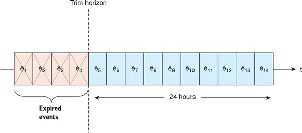
But there is a limit to this approach: neither Kafka nor Kinesis is intended to contain your entire event archive. In Kinesis, the trim horizon is set to 24 hours and can be increased up to 1 week (or 168 hours). After that cutoff, older events are trimmed—deleted from the stream forever. With Apache Kafka, the trim horizon (called the retention period) is also configurable: in theory, you could keep all your event data inside Kafka, but in practice, most people would limit their storage to one week (which is the default) or a month. Figure 7.1 depicts this limitation of our unified log.
Figure 7.1. The Kinesis trim horizon means that events in our stream are available for processing for only 24 hours after first being written to the stream.
As unified log programmers, the temptation is to say, “If data will be trimmed after some hours or days, let’s just make sure we do all of our processing before that time window is up!” For example, if we need to calculate certain metrics in that time window, let’s ensure that those metrics are calculated and safely written to permanent storage in good time. Unfortunately, this approach has key shortcomings; we could call these the Three Rs:
- Resilience
- Reprocessing
- Refinement
Let’s take these in turn.
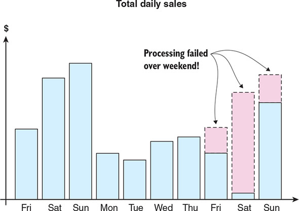
We want our unified log processing to be as resilient in the face of failure as possible. If we have Kinesis or Kafka set to delete events forever after 24 hours, that makes our event pipeline much more fragile: we must fix any processing failures before those events are gone from our unified log forever. If the problem happens over the weekend and we do not detect it, we are in trouble; there will be permanent gaps in our data that we have to explain to our boss, as visualized in figure 7.2.
Figure 7.2. A dashboard of daily sales annotated to explain the data missing from the second weekend. From the missing data, we can surmise that the outage started toward the end of Friday, continued through the weekend, and was identified and fixed on Monday (allowing most of Sunday’s data to be recovered).
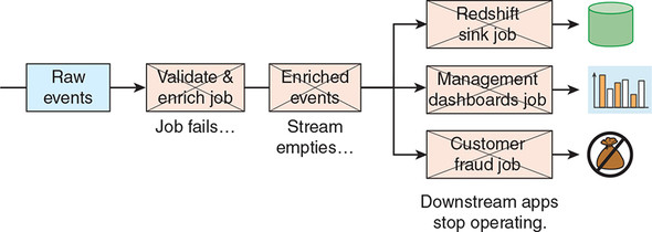
Remember too that our pipelines typically consist of multiple processing stages, so any stages downstream of our failure will also be missing important input data. We’ll have a cascade failure. Figure 7.3 demonstrates this cascade failure—our upstream job that validates and enriches our events fails, causing cascade failures in various downstream applications, specifically these:
- A stream processing job that loads the events into Amazon Redshift
- A stream processing job that provides management dashboards, perhaps similar to that visualized in figure 7.2
- A stream processing job that monitors the event stream looking for customer fraud
Figure 7.3. A failure in our upstream job that validates and enriches our event causes cascade failures in all of our downstream jobs, because the stream of enriched events that they depend on is no longer being populated.
Even worse, with Kinesis, the window we have to recover from failure is shorter than 24 hours. This is because, after the problem is fixed, we will have to resume processing events from the point of failure onward. Because we can read only up to 2 MB of data from each Kinesis shard per second, it may not be physically possible to process the entire backlog before some of it is trimmed (lost forever). In those cases, you might want to increase the trim horizon to the maximum allowed, which is 168 hours.
Because we cannot foresee and fix all the various things that could fail in our job, it becomes important that we have a robust backup of our incoming events. We can then use this backup to recover from any kind of stream processing failure at our own speed.
In chapter 5, we wrote a stream processing job in Samza that detected abandoned shopping carts after 30 minutes of customer inactivity. This worked well, but what if we have a nagging feeling that a different definition of cart abandonment might suit our business better? If we had all of our events stored somewhere safe, we could apply multiple different cart abandonment algorithms to that event archive, review the results, and then port the most promising algorithms into our stream processing job.
More broadly, there are several reasons that we might want to reprocess an event stream from a full archive of that stream:
- We want to fix a bug in an existing calculation or aggregation. For example, we find that our daily metrics are being calculated against the wrong time zone.
- We want to alter our definition of a metric. For example, we decide that a user’s browsing session on our website ends after 15 minutes of inactivity, not 30 minutes.
- We want to apply a new calculation or aggregation retrospectively. For example, we want to track cumulative e-commerce sales per device type as well as per country.
All of these use cases depend on having access to the event stream’s entire history—which, as you’ve seen, isn’t possible with Kinesis, and is somewhat impractical with Kafka.
Assuming that the calculations and aggregations in our stream processing job are bug-free, just how accurate will our job’s results be? They may not be as accurate as we would like, for three key reasons:
- Late-arriving data— At the time that our job is performing the calculation, it may not have access to all of the data that the calculation needs.
- Approximations— We may choose to use an approximate calculation in our stream processing job on performance grounds.
- Framework limitations— Architectural limitations may be built into our stream processing framework that impact the accuracy of our processing.
In the real world, data is often late arriving, and this has an impact on the accuracy of our stream processing calculations. Think of a mobile game that is sending to our unified log a stream of events recording each player’s interaction with the game.
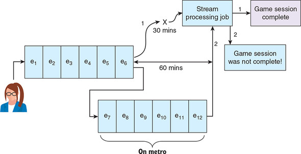
Say a player takes the city’s underground metro and loses signal for an hour. The player continues playing on the metro, and the game keeps faithfully recording events; the game then sends them the cached events in one big batch when the user gets above ground again. Unfortunately, while the user was underground, our stream processing job already decided that the player had finished playing the game and updated its metrics on completed game sessions accordingly. The late-arriving batch of events invalidates the conclusions drawn by our stream processing app, as visualized in figure 7.4.
Figure 7.4. Our stream processing job draws the wrong conclusion—that a game session has finished—because relevant events arrive too late to be included in the decision-making process.
The data that online advertising companies provide to their customers is another example. It takes days (sometimes weeks) for these companies to determine which clicks on ads were real and which ones were fraudulent. Therefore, it also takes days or weeks for marketing spend data to be finalized, sometimes referred to as becoming golden. As a result, any join we do in a stream processing job between our ad click and what we paid for that click will be only a first estimate, and subject to refinement using our late-arriving data.
For performance reasons, you may choose to make approximations in your stream processing algorithms. A good example, explored in Big Data, is calculating unique visitors to a website. Calculating unique visitors (COUNT DISTINCT in SQL) can be challenging because the metric is not additive—for example, you cannot calculate the number of unique visitors to a website in a month by adding together the unique visitor numbers for the constituent weeks. Because accurate uniqueness counts are computationally expensive, often we will choose an approximate algorithm such as HyperLogLog for our stream processing.[2]
2The HyperLogLog algorithm for approximating uniqueness counts is described at Wikipedia: https://en.wikipedia.org/wiki/HyperLogLog.
Although these approximations are often satisfactory for stream processing, an analytics team usually will want to have the option of refining those calculations. In the case of unique visitors to the website, the analytics team might want to be able to generate a true COUNT DISTINCT across the full history of website events.
This last reason is a hot topic in stream processing circles. Nathan Marz’s Lambda Architecture is designed around the idea that the stream processing component (what he calls the speed layer) is inherently unreliable.
A good example of this is the concept of exactly-once versus at-least-once processing, which has been discussed in chapter 5. Currently, Amazon Kinesis offers only at-least-once processing: an event will never be lost as it moves through a unified log pipeline, but it may be duplicated one or more times. If a unified log pipeline duplicates events, this is a strong rationale for performing additional refinement, potentially using a technology that supports exactly-once processing. It is worth noting, though, that as of release 0.11, Apache Kafka also supports exactly-once delivery semantics.
This is a hot topic because Jay Kreps, the original architect of Apache Kafka, disagrees that stream processing is inherently unreliable; he sees this more as a transitional issue with the current crop of unified log technologies.[3] He has called this the Kappa Architecture, the idea that we should be able to use a single stream-processing stack to meet all of our unified log needs.
3You can read more about Kreps’ ideas in his seminal article that coined the term “Kappa Architecture” at www.oreilly.com/ideas/questioning-the-lambda-architecture.
My view is that framework limitations will ultimately disappear, as Jay says. But late-arriving data and pragmatic approximation decisions will always be with us. And today these three accuracy issues collectively give us a strong case for creating and maintaining an event archive.
In the preceding section, you saw that archiving the event streams that flow through our unified log makes our processing architecture more robust, allows us to reprocess when needed, and lets us refine our processing outputs. In this section, we will look at the what, where, and how of event stream archiving.
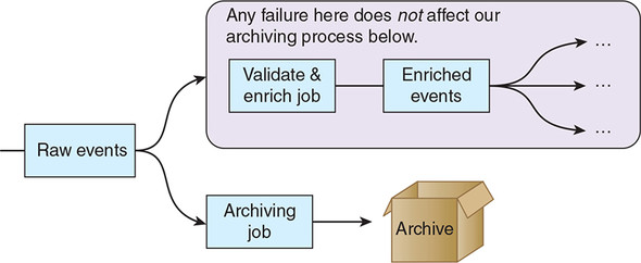
We have decided that archiving events within our unified log is a good idea, but what precisely should we be archiving? The answer may not be what you are expecting: you should archive the rawest events you can, as far upstream in your event pipeline as possible. This early archiving is shown in figure 7.5, which builds on the unified log topology set out earlier in figure 7.3.
Figure 7.5. By archiving as far upstream as possible, we insulate our archiving process from any failures that occur downstream of the raw event stream.
- In chapters 2 and 3, we would archive the three types of events generated by shoppers on the Nile website.
- In chapter 5, we would archive the health-check event generated by the machines on Plum’s production line.
Event validation and enrichment can be a costly process, so why insist on archiving the rawest events? Again, it comes down to the three Rs:
- Resilience— By archiving as upstream as possible, we are guaranteeing that there are no intermediate stream-processing jobs that could break and thus cause our archiving to fail.
- Reprocessing— We may want to reprocess any part of our event pipeline—yes, even the initial validation and enrichment jobs. By having the rawest events archived, we should be able to reprocess anything downstream.
- Refinement— Any refinement process (such as a Hadoop or Spark batch-processing job) should start from the exact same input events as the stream processing job that it aims to refine.
We need to archive our event stream to permanent file storage that has the following characteristics:
- Is robust, because we don’t want to learn later that parts of the archive have been lost
- Makes it easy for data processing frameworks such as Hadoop or Spark to quickly load the archived events for further processing or refinement
Both requirements point strongly to a distributed filesystem. Table 7.1 lists the most popular examples; our rawest event stream should be archived to at least one of these.
Table 7.1. Examples of distributed filesystems (view table figure)
Your choice of storage will be informed by whether your company uses an infrastructure-as-a-service (IaaS) offering such as AWS, Azure, or Google Compute Engine, or has built its own data processing infrastructure. But even if your company has built its own private infrastructure, you may well choose to archive your unified log to a hosted service such as Amazon S3 as well, as an effective off-site backup.
The fundamentals of archiving events from our unified log into our permanent file storage are straightforward. We need a stream consumer that does the following:
- Reads from each shard or topic in our stream
- Batches a sensible number of events into a file that is optimized for subsequent data processing
- Writes each file to our distributed filesystem of choice
The good news is that this is a solved problem, so we won’t have to write any code just yet! Various companies have open sourced tools to archive either Kafka or Kinesis event streams to one or other of these distributed filesystems. Table 7.2 itemizes the most well-known of these.
Table 7.2. Tools for archiving our unified log from a distributed filesystem (view table figure)
| Tool |
From |
To |
Creator |
Description |
|---|---|---|---|---|
| Camus | Kafka | HDFS | A MapReduce job that loads Kafka into HDFS. Can autodiscover Kafka topics. | |
| Flafka | Kafka | HDFS | Cloudera / Flume | Part of the Flume project. Involves configuring a Kafka source plus HDFS sink. |
| Bifrost | Kafka | S3 | uSwitch.com | Writes events to S3 in uSwitch.com’s own baldr binary file format. |
| Secor | Kafka | S3 | A service for persisting Kakfa topics to S3 as Hadoop SequenceFiles. | |
| kinesis-s3 | Kinesis | S3 | Snowplow | A Kinesis Client Library application to write a Kinesis stream to S3. |
| Connect S3 | Kafka | S3 | Confluent | Allows exporting data from Kafka topics to S3 objects in either Avro or JSON formats. |
Now that you understand the why and how of archiving our raw event stream, we will put the theory into practice by using one of these tools: Pinterest’s Secor.
Let’s return to Nile, our online retailer from chapter 5. Remember that Nile’s shoppers generate three types of events, all of which are collected by Nile and written to their Apache Kafka unified log. The three event types are as follows:
- Shopper views product
- Shopper adds item to cart
- Shopper places order
Alongside the existing stream processing we are doing on these events, Nile wants to archive all of these events to Amazon S3. Figure 7.6 sets out the desired end-to-end architecture.
Figure 7.6. Alongside Nile’s three existing stream-processing applications, we will be adding a fourth application, which archives the raw event stream to Amazon S3.
;%22/%3E%3C/svg%3E)
Looking at the various archiving tools in table 7.2, the only three that fit the bill for archiving Kafka to Amazon S3 are uSwitch’s Bifrost, Pinterest’s Secor, and Confluent’s Kafka Connect S3. For Nile, we choose Secor over Bifrost because Secor’s storage format—Hadoop SequenceFiles—is much more widely adopted than Bifrost’s baldr format. Remember, Nile will want to mine the event data stored in its S3 archive for many years to come, so it’s crucial that we use non-niche data formats that will be well supported for the foreseeable future. We also could have chosen Confluent’s Kafka Connect S3, but that would require us to install Confluent’s Kafka distribution instead of Apache’s. Because we already have the latter running, let’s get started with that.
First, we need to get Nile’s raw events flowing into Kafka again. Assuming you still have Kafka deployed as per chapter 2, you can start up Apache ZooKeeper again like so:
$ cd kafka_2.12-2.0.0
$ bin/zookeeper-server-start.sh config/zookeeper.properties
Now we are ready to start Kafka in a second terminal:
$ cd kafka_2.12-2.0.0
$ bin/kafka-server-start.sh config/server.properties
Let’s create the raw-events-ch07 topic in Kafka as we did in chapter 5, so we can send some events in straightaway. You can make that topic available in Kafka by creating it like this:
$ bin/kafka-topics.sh --create --topic raw-events-ch07 \
  --zookeeper localhost:2181 --replication-factor 1 --partitions 1
Created topic "raw-events-ch07".
Now in your third terminal, run the Kafka console producer like so:
$ bin/kafka-console-producer.sh \
    --broker-list localhost:9092 --topic raw-events-ch07
This producer will sit waiting for input. Let’s feed it some events, making sure to press Enter after every line:
{ "subject": { "shopper": "789" }, "verb": "add", "indirectObject":
 "cart", "directObject": { "item": { "product": "aabattery", "quantity":
 12, "price": 1.99 }}, "context": { "timestamp": "2018-10-30T23:01:29" } }

{ "subject": { "shopper": "456" }, "verb": "add", "indirectObject":
 "cart", "directObject": { "item": { "product": "thinkpad", "quantity":
 1, "price": 1099.99 }},"context": { "timestamp": "2018-10-30T23:03:33" }}

{ "subject": { "shopper": "789" }, "verb": "add", "indirectObject":
 "cart", "directObject": { "item": { "product": "ipad", "quantity": 1,
 "price": 499.99 } }, "context": { "timestamp": "2018-10-30T00:04:41" } }

{ "subject": { "shopper": "789" }, "verb": "place", "directObject":
 { "order": { "id": "123", "value": 511.93, "items": [ { "product":
 "aabattery", "quantity": 6 }, { "product": "ipad", "quantity": 1} ] } },
 "context": { "timestamp": "2018-10-30T00:08:19" } }

{ "subject": { "shopper": "123" }, "verb": "add", "indirectObject":
 "cart", "directObject": { "item": { "product": "skyfall", "quantity":
 1, "price": 19.99 }}, "context": { "timestamp": "2018-10-30T00:12:31" } }

{ "subject": { "shopper": "123" }, "verb": "add", "indirectObject":
 "cart", "directObject": { "item": { "product": "champagne", "quantity":
 5, "price": 59.99 }}, "context": { "timestamp": "2018-10-30T00:14:02" } }

{ "subject": { "shopper": "123" }, "verb": "place", "directObject":
 { "order": { "id": "123", "value": 179.97, "items": [ { "product":
 "champagne", "quantity": 3 } ] } }, "context": { "timestamp":
 "2018-10-30T00:17:18" } }
Phew! After entering all of these, you can now press Ctrl-D to exit the console producer. It’s a little hard to tell from all those JSON objects exactly what is happening on the Nile website. Figure 7.7 illustrates the three shoppers who are adding these products to their carts and then placing their orders.
Figure 7.7. Our seven events visualized: three shoppers are adding products to their basket; two of those shoppers are going on to place orders, but with reduced quantities in their baskets.
;%22/%3E%3C/svg%3E)
In any case, those seven events should all be safely stored in Kafka now, and we can check this easily using the console consumer:
$ bin/kafka-console-consumer.sh --topic raw-events-ch07 --from-beginning \
    --bootstrap-server localhost:9092
{ "subject": { "shopper": "789" }, "verb": "add", "indirectObject":
 "cart", "directObject": { "item": { "product": "aabattery", "quantity":
 12, "unitPrice": 1.99 } }, "context": { "timestamp":
 "2018-10-30T23:01:2" } }
...
Then press Ctrl-C to exit the consumer. Great—our events have been safely logged in Kafka, so we can move on to the archiving.
Remember that Nile wants all of the raw events that are being written to Kafka to be archived to Amazon Simple Storage Service, more commonly referred to as Amazon S3. From earlier in part 2, you should be comfortable with Amazon Web Services, although we have yet to use Amazon S3.
In chapter 4, we created an Amazon Web Services user called ulp, and gave that user full permissions on Amazon Kinesis. We now need to log back into the AWS as our root user and assign the ulp user full permissions on Amazon S3. From the AWS dashboard:
- Click the Identity & Access Management icon.
- Click the Users option in the left-hand navigation pane.
- Click your ulp user.
- Click the Add Permissions button.
- Click the Attach Existing Policies Directly tab.
- Select the AmazonS3FullAccess policy and click Next: Review.
- Click the Add Permissions button.
We are now ready to create an Amazon S3 bucket to archive our events into. An S3 bucket is a top-level folder-like resource, into which we can place individual files. Slightly confusingly, the names of S3 buckets have to be globally unique. To prevent your bucket’s name from clashing with that of other readers of this book, let’s adopt a naming convention like this:
s3://ulp-ch07-archive-{{your-first-pets-name}}
Use the AWS CLI tool’s s3 command and mb (for make bucket) subcommand to create your new bucket, like so:
$ aws s3 mb s3://ulp-ch07-archive-little-torty --profile=ulp
make_bucket: s3://ulp-ch07-archive-little-torty/
Our bucket has been created. We now have our shopper events sitting in Kafka and an empty bucket in Amazon S3 ready to archive our events in. Let’s add in Secor and connect the dots.
There are no prebuilt binaries for Secor, so we will have to build it from source ourselves. The Vagrant development environment has all the tools we need to get started:
$ cd /vagrant
$ wget https://github.com/pinterest/secor/archive/v0.26.tar.gz
$ cd secor-0.26
Next, we need to edit the configuration files that Secor will run against. First, load this file in your editor of choice:
/vagrant/secor/src/main/config/secor.common.properties
Now update the settings within the MUST SET section, as in the following listing.
Listing 7.1. secor.common.properties
...
# Regular expression matching names of consumed topics.
secor.kafka.topic_filter=raw-events-ch07                   #1

# AWS authentication credentials.
aws.access.key={{access-key}}                              #2
aws.secret.key={{secret-key}}                              #3
...
Next you need to edit this file:
/vagrant/secor/src/main/config/secor.dev.properties
We have only one setting to change here: the secor.s3.bucket property. This needs to match the bucket that we set up in section 7.3.2. When that’s done, your secor.dev.properties file should look similar to that set out in the following listing.
Listing 7.2. secor.dev.properties
include=secor.common.properties                             #1

############
# MUST SET #
############

# Name of the s3 bucket where log files are stored.
secor.s3.bucket=ulp-ch07-archive-{{your-first-pets-name}}   #2

################
# END MUST SET #
################

kafka.seed.broker.host=localhost
kafka.seed.broker.port=9092

zookeeper.quorum=localhost:2181

# Upload policies.                                         #3
# 10K
secor.max.file.size.bytes=10000
# 1 minute
secor.max.file.age.seconds=60
From this listing, we can see that the default rules for uploading our event files to S3 are to wait for either 1 minute or until our file contains 10,000 bytes, whichever comes sooner. These defaults are fine, so we will leave them as is. And that’s it; we can leave the other configuration files untouched and move on to building Secor:
$ mvn package
...
[INFO] BUILD SUCCESS...
...
$ sudo mkdir /opt/secor
$ sudo tar -zxvf target/secor-0.26-SNAPSHOT-bin.tar.gz -C /opt/secor
...
lib/jackson-core-2.6.0.jar
lib/java-statsd-client-3.0.2.jar
Finally, we are ready to run Secor:
$ sudo mkdir -p /mnt/secor_data/logs
$ cd /opt/secor
$ sudo java -ea -Dsecor_group=secor_backup \
    -Dlog4j.configuration=log4j.prod.properties \
    -Dconfig=secor.dev.backup.properties -cp \
    secor-0.26.jar:lib/* com.pinterest.secor.main.ConsumerMain
Nov 05, 2018 11:26:32 PM com.twitter.logging.Logger log
INFO: Starting LatchedStatsListener
...
INFO: Cleaning up!
Note that some few seconds will elapse before the final INFO: Cleaning up! message appears; in this time, Secor is finalizing the batch of events, storing it in a Hadoop SequenceFile, and uploading it to Amazon S3.
Let’s quickly check that the file has successfully uploaded to S3. From the AWS dashboard:
- Click the S3 icon.
- Click the bucket ulp-ch07-archive-{{your-first-pets-name}}.
- Click each subfolder until you arrive at a single file.
This file contains our seven events, read from Kafka and successfully uploaded to S3 by Secor, as you can see in figure 7.8.
;%22/%3E%3C/svg%3E)
We can download the archived file by using the AWS CLI tools:
$ cd /tmp
$ PET=little-torty
$ FILE=secor_dev/backup/raw-events-ch07/offset=0/1_0_00000000000000000000
$ aws s3 cp s3://ulp-ch07-archive-${PET}/${FILE} . --profile=ulp
download: s3://ulp-ch07-archive-little-torty/secor_dev/backup/raw-events-
ch07/offset=0/1_0_00000000000000000000 to ./1_0_00000000000000000000
What’s in the file? Let’s have a quick look inside it:
$ file 1_0_00000000000000000000
1_0_00000000000000000000: Apache Hadoop Sequence file version 6
$ $ head -1 1_0_00000000000000000000
SEQ!org.apache.hadoop.io.LongWritable"org.a pache.hadoop.io.BytesWritabl...
Alas, we can’t easily read the file from the command line. The file is stored by Secor as a Hadoop SequenceFile, which is a flat file format consisting of binary key-value pairs.[4] Batch processing frameworks such as Hadoop can easily read SequenceFiles, and that is what we’ll explore next.
4A definition of the Hadoop SequenceFile format is available at https://wiki.apache.org/hadoop/SequenceFile.
Now that we have our raw events safely archived in Amazon S3, we can use a batch processing framework to process these events in any way that makes sense to Nile.
The fundamental difference between batch processing frameworks and stream processing frameworks relates to the way in which they ingest data. Batch processing frameworks expect to be run against a terminated set of records, unlike the unbounded event stream (or streams) that a stream-processing framework reads. Figure 7.9 illustrates a batch processing framework.
Figure 7.9. A batch processing framework has processed four distinct batches of events, each belonging to a different day of the week. The batch processing framework runs at 3 a.m. daily, ingests the data for the prior day from storage, and writes its outputs back to storage at the end of its run.
;%22/%3E%3C/svg%3E)
By way of comparison, figure 7.10 illustrates how a stream processing framework works on an unterminated stream of events.
Figure 7.10. A stream processing framework doesn’t distinguish any breaks in the incoming event stream. Monday through Thursday’s data exists as one unbounded stream, likely with overlap due to late-arriving events.
;%22/%3E%3C/svg%3E)
A second, perhaps more historical, difference is that batch processing frameworks have been used with a much broader variety of data than stream processing frameworks. The canonical example for batch processing as popularized by Hadoop is counting words in a corpus of English-language documents (semistructured data). By contrast, stream processing frameworks have been more focused on well-structured event stream data, although some promising initiatives support processing other data types in stream.[5]
5An experimental initiative to integrate Luwak within Samza can be found at https://github.com/romseygeek/samza-luwak.
Table 7.3 lists the major distributed batch-processing frameworks. Of these, Apache Hadoop and, increasingly, Apache Spark are far more widely used than Disco or Apache Flink.
Table 7.3. Examples of distributed batch-processing frameworks (view table figure)
| Framework |
Started |
Creator |
Description |
|---|---|---|---|
| Disco | 2008 | Nokia Research Center | MapReduce framework written in Erlang. Has its own filesystem, DDFS. |
| Apache Flink | 2009 | TU Berlin | Formerly known as Project Stratosphere, Flink is a streaming dataflow engine with a DataSet API for batch processing. Write jobs in Scala, Java, or Python. |
| Apache Hadoop | 2008 | Yahoo! | Software framework written in Java for distributed processing (Hadoop MapReduce) and distributed storage (HDFS). |
| Apache Spark | 2009 | UC Berkeley AMPLab | Large-scale data processing, supporting cyclic data flow and optimized for memory use. Write jobs in Scala, Java, or Python. |
What do we mean when we say that these frameworks are distributed? Simply put, we mean that they have a master-slave architecture:
- The master supervises the slaves and parcels out units of work to the slaves.
- The slaves (sometimes called workers) receive the units of work, perform them, and provide status updates to the master.
Figure 7.11 represents this architecture. This distribution allows processing to scale horizontally, by adding more slaves.
Figure 7.11. In a distributed data-processing architecture, the master supervises a set of slaves, allocating them units of work from the batch processing job.
;%22/%3E%3C/svg%3E)
The analytics team at Nile wants a report on the lifetime behavior of every Nile shopper:
- How many items has each shopper added to their basket, and what is the total value of all items added to basket?
- Similarly, how many orders has each shopper placed, and what is the total value of each shopper’s orders?
Figure 7.12 shows a sample report.
Figure 7.12. For each shopper, the Nile analytics team wants to know the volume and value of items added to basket, and the volume and value of orders placed. With this data, the value of abandoned carts is easily calculated.
;%22/%3E%3C/svg%3E)
If we imagine that the Nile analytics team came up with this report six months into us operating our event archive, we can see that this is a classic piece of reprocessing: Nile wants us to apply new aggregations retrospectively to the full event history.
Before we write a line of code, let’s come up with the algorithms required to produce this report. We will use SQL-esque syntax to describe the algorithms. Here’s an algorithm for the shoppers’ add-to-basket activity:
GROUP BY shopper_id
WHERE event_type IS add_to_basket
  items = SUM(item.quantity)
  value = SUM(item.quantity * item.price)
We calculate the volume and value of items added to each shopper’s basket by looking at the Shopper adds item to basket events. For the volume of items, we sum all of the item quantities recorded in those events. Value is a little more complex: we have to multiply all of the item quantities by the item’s unit price to get the total value.
GROUP BY shopper_id
WHERE event_type IS place_order
  orders = COUNT(rows)
  value  = SUM(order.value)
For each shopper, we look at their Shopper places order events only. A simple count of those rows tells us the number of orders they have placed. A sum of the values of those orders gives us the total amount they have spent.
And that’s it. Now that you know what calculations we want to perform, we are ready to pick a batch processing framework and write them.
We need to choose a batch processing framework to write our job in. We will use Apache Spark: it has an elegant Scala API for writing the kinds of aggregations that we require, and it plays relatively well with Amazon S3, where our event archive lives, and Amazon Elastic MapReduce (EMR), which is where we will ultimately run our job. Another plus for Spark is that it’s easy to build up our processing job’s logic interactively by using the Scala console.
Let’s get started. We are going to create our Scala application by using Gradle. First, create a directory called spark, and then switch to that directory and run the following:
$ gradle init --type scala-library
...
BUILD SUCCESSFUL
...
As we did in previous chapters, we’ll now delete the stubbed Scala files that Gradle created:
$ rm -rf src/*/scala/*
The default build.gradle file in the project root isn’t quite what we need either, so replace it with the code in the following listing.
Listing 7.3. build.gradle
apply plugin: 'scala'

configurations {                                                      #1
    provided
}

sourceSets {                                                          #1
    main.compileClasspath += configurations.provided
}

repositories {
  mavenCentral()
}

version = '0.1.0'

 ScalaCompileOptions.metaClass.daemonServer = true
 ScalaCompileOptions.metaClass.fork = true
 ScalaCompileOptions.metaClass.useAnt = false
 ScalaCompileOptions.metaClass.useCompileDaemon = false

dependencies {
  runtime "org.scala-lang:scala-compiler:2.12.7"
  runtime "org.apache.spark:spark-core_2.12:2.4.0"
  runtime "org.apache.spark:spark-sql_2.12:2.4.0"
  compile "org.scala-lang:scala-library:2.12.7"
  provided "org.apache.spark:spark-core_2.12:2.4.0"                   #2
  provided "org.apache.spark:spark-sql_2.12:2.4.0"
}

jar {
  dependsOn configurations.runtime
  from {
    (configurations.runtime - configurations.provided).collect {      #3
      it.isDirectory() ? it : zipTree(it)
    }
  } {
    exclude "META-INF/*.SF"
    exclude "META-INF/*.DSA"
    exclude "META-INF/*.RSA"
  }
}

task repl(type:JavaExec) {                                            #4
    main = "scala.tools.nsc.MainGenericRunner"
    classpath = sourceSets.main.runtimeClasspath
    standardInput System.in
    args '-usejavacp'
}
With that updated, let’s just check that everything is still functional:
$ gradle build
...
BUILD SUCCESSFUL
One last piece of housekeeping before we start coding—let’s copy the Secor SequenceFile that we downloaded from S3 at the end of section 7.3 to a data subfolder:
$ mkdir data
$ cp ../1_0_00000000000000000000 data/
Okay, good. Now let’s write some Scala code! Still in the project root, start up the Scala console or REPL with this command:
$ gradle repl --console plain
...
scala>
Note that if you have Spark already installed on your local computer, you might want to use spark-shell instead.[6] Before we write any code, let’s pull in imports that we need. Type the following into the Scala console (we have omitted the scala> prompt and the console’s responses for simplicity):
6The Spark shell is a powerful tool to analyze data interactively: https://spark.apache.org/docs/latest/quick-start.html#interactive-analysis-with-the-spark-shell.
import org.apache.spark.{SparkContext, SparkConf}
import SparkContext._
import org.apache.spark.sql._
import functions._
import org.apache.hadoop.io.BytesWritable
Next, we need to create a SparkConf, which configures the kind of processing environment we want our job to run in. Paste this into your console:
val spark = SparkSession.builder()
  .appName("ShopperAnalysis")
  .master("local")
  .getOrCreate()
Feeding this configuration into a new SparkContext will cause Spark to boot up in our console:
scala> val sparkContext = spark.sparkContext
...
sparkContext: org.apache.spark.SparkContext =
 org.apache.spark.SparkContext@3d873a97
Next, we need to load the events file archived to S3 by Secor. Assuming this is in your data subfolder, you can load it like this:
scala> val file = sparkContext.
  sequenceFile[Long, BytesWritable]("./data/1_0_00000000000000000000")
...
file:org.apache.spark.rdd.RDD[(Long, org.apache.hadoop.io.BytesWritable)]
 = MapPartitionsRDD[1] at sequenceFile at <console>:23
Remember that a Hadoop SequenceFile is a binary key-value file format: in Secor’s case, the key is a Long number, and the value is our event’s JSON converted to a BytesWritable, which is a Hadoop-friendly byte array. The type of our file variable is now an RDD[(Long, BytesWritable)]; RDD is a Spark term, short for a resilient distributed dataset. You can think of the RDD as a way of representing the structure of your distributed collection of items at that point in the processing pipeline.
This RDD[(Long, BytesWritable)] is a good start, but really we just want to be working with human-readable JSONs in String form. Fortunately, we can convert the RDD to exactly this by applying this function to each of the values, by mapping over the collection:
scala> val jsons = file.map { case (_, bw) =>
  new String(bw.getBytes, 0, bw.getLength, "UTF-8")
}
jsons: org.apache.spark.rdd.RDD[String] = MapPartitionsRDD[2] at map
 at <console>:21
Note the return type: it’s now an RDD[String], which is what we wanted. We’re almost ready to write our aggregation code! Spark has a dedicated module, called Spark SQL (https://spark.apache.org/sql/), which we can use to analyze structured data such as an event stream. Spark SQL is a little confusingly named—we can use it without writing any SQL. First, we have to create a new SqlContext from our existing SparkContext:
val sqlContext = spark.sqlContext
A Spark SQLContext has a method on it to create a JSON-flavored data structure from a vanilla RDD, so let’s employ that next:
scala> val events = sqlContext.read.json(jsons)
18/11/05 07:45:53 INFO FileInputFormat: Total input paths to process : 1
...
18/11/05 07:45:56 INFO DAGScheduler: Job 0 finished: json at <console>:24,
 took 0.376407 s
events: org.apache.spark.sql.DataFrame = [context: struct<timestamp:
 string>, directObject: struct<item: struct<price: double, product: string
 ... 1 more field>, order: struct<id: string, items:
 array<struct<product:string,quantity:bigint>> ... 1 more field>> ... 3
 more fields]
That’s interesting—Spark SQL has processed all of the JSON objects in our RDD[String] and automatically created a data structure containing all of the properties it found! Note too that the output structure is now something called a DataFrame, not an RDD. If you have ever worked with the R programming language or with the Pandas data analytics library for Python, you will be familiar with data frames: they represent a collection of data organized into named columns. Where Spark-proper still leans heavily on the RDD type, Spark SQL embraces the new DataFrame type.[7]
7You can read more about this topic in “Introducing DataFrames in Apache Spark for Large-Scale Data Science,” by Reynold Xin et al.: https://databricks.com/blog/2015/02/17/introducing-dataframes-in-spark-for-large-scale-data-science.html.
We are now ready to write our aggregation code. To make the code more readable, we’re going to define some aliases in Scala:
val (shopper, item, order) =
  ("subject.shopper", "directObject.item", "directObject.order")
These three aliases give us more convenient short-forms to refer to the three entities in our event JSON objects that we care about. Note that Spark SQL provides a dot-operator syntax to let us access a JSON property that is inside another property (as, for example, the shopper is inside the subject).
Now let’s run our aggregation code:
scala> events.
  filter(s"${shopper} is not null").
  groupBy(shopper).
  agg(
    col(shopper),
    sum(s"${item}.quantity"),
    sum(col(s"${item}.quantity") * col(s"${item}.price")),
    count(order),
    sum(s"${order}.value")
  ).collect
18/11/05 08:00:58 INFO CodeGenerator: Code generated in 14.294398 ms
...
18/11/05 08:01:07 INFO DAGScheduler: Job 1 finished: collect at
 <console>:43, took 1.315203 s
res0: Array[org.apache.spark.sql.Row] =
 Array([789,789,13,523.87,1,511.93], [456,456,1,1099.99,0,null],
 [123,123,6,319.94,1,179.97])
The collect at the end of our code forces Spark to evaluate our RDD and output the result of our aggregations. As you can see, the result contains three rows of data, in a slightly reader-hostile format. The three rows all match the table format depicted in figure 7.12: the cells consist of a shopper ID, add-to-basket items and value, and finally the number of orders and order value.
A few notes on the aggregation code itself:
- We filter out events with no shopper ID. This is needed because the Spark SequenceFile loader returns the file’s empty header row, as well as our seven valid event JSON objects.
- We group by the shopper ID, and include that field in our results.
- We compose our aggregations out of various Spark SQL helper functions, including col() for column name, sum() for a sum of values across rows, and count() for a count of rows.
And that completes our experiments in writing a Spark job at the Scala console! You have seen that we can build a sophisticated report for the Nile analytics team by using Spark SQL. But running this inside a Scala console isn’t a realistic option for the long-term, so in the next section we will look briefly at operationalizing this code by using Amazon’s Elastic MapReduce platform.
Setting up and maintaining a cluster of servers for batch processing is a major effort, and not everybody has the need or budget for an always-running (persistent) cluster. For example, if Nile wants only a daily refresh of the shopper spend analysis, we could easily achieve this with a temporary (transient) cluster that spins up at dawn each day, runs the job, writes the results to Amazon S3, and shuts down. Various data-processing-as-as-a-service offerings have emerged to meet these requirements, including Amazon Elastic MapReduce (EMR), Quobole, and Databricks Cloud.
Given that we already have an AWS account, we will use EMR to operationalize our job in this section. But before we can productionize our job, we first need to consolidate all of our code from the Scala console into a standalone Scala file. Copy the code from the following listing and add it into this file:
src/main/scala/nile/ShopperAnalysisJob.scala
The code in ShopperAnalysisJob.scala is functionally equivalent to the code we ran in the previous section. The main differences are as follows:
- We have improved readability a little (for example, by moving the byte wrangling for Secor’s SequenceFile format into a dedicated function, toJson).
- We have created a main, ready for Elastic MapReduce to call, and we are passing in arguments to specify the input file and the output folder.
- Our SparkConf looks somewhat different; these are the settings required to run the job in a distributed fashion on EMR.
- Instead of running collect as before, we are now using the saveAsTextFile method to write our results back into the output folder.
Listing 7.4. ShopperAnalysisJob.scala
package nile

import org.apache.spark.{SparkContext, SparkConf}
import SparkContext._
import org.apache.spark.sql._
import functions._
import org.apache.hadoop.io.BytesWritable

object ShopperAnalysisJob {

  def main(args: Array[String]) {

    val (inFile, outFolder) = {                                     #1
      val a = args.toList
      (a(0), a(1))
    }

  val sparkConf = new SparkConf()
    .setAppName("ShopperAnalysis")
    .setJars(List(SparkContext.jarOfObject(this).get))              #2
  val spark = SparkSession.builder()
    .config(sparkConf)
    .getOrCreate()
  val sparkContext = spark.sparkContext

  val file = sparkContext.sequenceFile[Long, BytesWritable](inFile)
  val jsons = file.map {
    case (_, bw) => toJson(bw)
  }

  val sqlContext = spark.sqlContext
  val events = sqlContext.read.json(jsons)

  val (shopper, item, order) =
    ("subject.shopper", "directObject.item", "directObject.order")
  val analysis = events
    .filter(s"${shopper} is not null")
    .groupBy(shopper)
    .agg(
      col(shopper),
      sum(s"${item}.quantity"),
      sum(col(s"${item}.quantity") * col(s"${item}.price")),
      count(order),
      sum(s"${order}.value")
    )

    analysis.rdd.saveAsTextFile(outFolder)                         #3
  }

  private def toJson(bytes: BytesWritable): String =               #4
    new String(bytes.getBytes, 0, bytes.getLength, "UTF-8")
}
Now we are ready to assemble our Spark job into a fat jar—in fact, this jar is not so fat, as the only dependency we need to bundle into the jar is the Scala standard library; the Spark dependencies are already available on Elastic MapReduce, which is why we flagged those dependencies as provided. Build the fat jar from the command line like so:
$ gradle jar
:compileJava UP-TO-DATE
:compileScala UP-TO-DATE
:processResources UP-TO-DATE
:classes UP-TO-DATE
:jar

BUILD SUCCESSFUL

Total time: 3 mins 40.261 secs
$ file build/libs/spark-0.1.0.jar
build/libs/spark-0.1.0.jar: Zip archive data, at least v1.0 to extract
To run this job on Elastic MapReduce, we first have to make the fat jar available to the EMR platform. This is easy to do; we can simply upload the file to a new folder, jar, in our existing S3 bucket:
$ aws s3 cp build/libs/spark-0.1.0.jar s3://ulp-ch07-archive-${PET}/jar/ \
 --profile=ulp
upload: build/libs/spark-0.1.0.jar to s3://ulp-ch07-archive-little-
torty/jar/spark-0.1.0.jar
Before we can run the job, we need to log back into the AWS as our root user and assign the ulp user full administrator permissions; this is because our ulp user will need wide-ranging permissions in order to prepare the account for running EMR jobs. From the AWS dashboard:
- Click the Identity & Access Management icon.
- Click Users in the left-hand navigation pane.
- Click your ulp user.
- Click the Add Permissions button.
- Click the Attach Existing Policies Directly tab.
- Select the AdministratorAccess policy and click Next: Review.
- Click the Add Permissions button.
Before we can run our job, we need to create an EC2 keypair plus IAM security roles for Elastic MapReduce to use. From inside your virtual machine, enter the following:
$ aws emr create-default-roles --profile=ulp --region=eu-west-1
$ aws ec2 create-key-pair --key-name=spark-kp --profile=ulp \
  --region=eu-west-1
This will create the new security roles required by Elastic MapReduce to run a job. Now run this:
$ BUCKET=s3://ulp-ch07-archive-${PET}
$ IN=${BUCKET}/secor_dev/backup/raw-events-
 ch07/offset=0/1_0_00000000000000000000
$ OUT=${BUCKET}/out
$ aws emr create-cluster --name Ch07-Spark --ami-version 3.6 \
--instance-type=m3.xlarge --instance-count 3 --applications Name=Hive \
--use-default-roles --ec2-attributes KeyName=spark-kp \
--log-uri ${BUCKET}/log --bootstrap-action \
 Name=Spark,Path=s3://support.elasticmapreduce/spark/install-spark,
 Args=[-x] --steps Name=ShopperAnalysisJob,Jar=s3://eu-west-1.
 elasticmapreduce/libs/script-runner/script-runner.jar,
 Args=[/home/hadoop/spark/bin/spark-submit,--deploy-mode,cluster,
 --master,yarn-cluster,--class,nile.ShopperAnalysisJob,
${BUCKET}/jar/spark-0.1.0.jar,${IN},${OUT}] \
--auto-terminate --profile=ulp --region=eu-west-1
{
    "ClusterId": "j-2SIN23GBVJ0VM"
}
The last three lines—the JSON containing the cluster ID—tell us that the cluster is now starting up. Before we take a look at the cluster, let’s break down the preceding create-cluster command into its constituent parts:
- Start an Elastic MapReduce cluster called Ch07-Spark using the default EMR roles.
- Start up three m3.xlarge instances (one master and two slaves) running AMI version 3.6.
- Log everything to a log subfolder in our bucket.
- Install Hive and Spark onto the cluster.
- Add a single job step, nile.ShopperAnalysisJob, as a Spark job found inside the jar/spark-0.1.0.jar file in our bucket.
- Provide the in-file and out-folder as first and second arguments to our job, respectively.
- Terminate the cluster when the Spark job step is completed.
A bit of a mouthful! In any case, we can now go and watch our cluster starting up. From the AWS dashboard:
- Make sure you have the Ireland region selected at the top right (or the region you’ve specified when provisioning the cluster).
- In the Analytics section, click EMR.
- In your Cluster List, click the job called Ch07-Spark.
You should see EMR first provisioning the cluster, and then bootstrapping the servers with the required software, as per figure 7.13.
Figure 7.13. Our new Elastic MapReduce cluster is running bootstrap actions on both our master and slave (aka core) instances.
;%22/%3E%3C/svg%3E)
Wait a little while, and the job status should change to Running. At this point, scroll down to the Steps subsection and expand both job steps, Install Hive and ShopperAnalysisJob. You can now watch these steps running, as shown in figure 7.14.
Figure 7.14. Our cluster has successfully completed running two job steps: the first step installed Hive on the cluster, while the second ran our Spark ShopperAnalysisJob. This is a helpful screen for debugging any failures in the operation of our steps.
If everything has been set up correctly, each step’s status should move to Completed, and then the overall cluster’s status should move to Terminated, All Steps Completed. We can now admire our handiwork:
$ aws s3 ls ${OUT}/ --profile=ulp
2018-11-05 08:22:35          0 _SUCCESS
2018-11-05 08:22:30          0 part-00000
...
2018-11-05 08:22:30         25 part-00017
...
2018-11-05 08:22:31         23 part-00038
...
2018-11-05 08:22:31         24 part-00059
...
2018-11-05 08:22:35          0 part-00199
The _SUCCESS is a slightly old-school flag file: an empty file whose arrival tells any downstream process that is monitoring this folder that no more files will be written to this folder. The more interesting output is our part- files. Collectively, these files represent the output to our Spark job. Let’s download them and review the contents:
$ aws s3 cp ${OUT}/ ./data/ --recursive --profile=ulp
...
download: s3://ulp-ch09-archive-little-torty/out/_SUCCESS to data/_SUCCESS
...
download: s3://ulp-ch09-archive-little-torty/out/part-00196 to
 data/part-00196
$ cat ./data/part-00*
[789,13,499.99,1,511.93]
[456,1,1099.99,0,null]
[123,6,319.94,1,179.97]
And there are our results! Don’t worry about the number of empty part- files created; that is an artifact of the way Spark is dividing its processing work into smaller work units. The important thing is that we have managed to transfer our Spark job to running on a remote, transient cluster of servers, completely automated for us by Elastic MapReduce.
If Nile were a real company, the next step for us would be to automate the operation of this job further, potentially using the following:
- A library for running and monitoring the job, such as boto (Python), Elasticity (Ruby), Spark Plug (Scala), or Lemur (Clojure)
- A tool for scheduling the job to run overnight, such as cron, Jenkins, or Chronos
We leave those as exercises to you! The important thing is that you have seen how to develop a batch processing job locally by using the Scala console/REPL, and then how to put that job into operation on a remote server cluster using Elastic MapReduce. Almost everything else in batch processing is just a variation on this theme.
- A unified log such as Apache Kafka or Amazon Kinesis is not designed as a long-term store of events. Kinesis has a hard limit, or trim horizon, of a maximum of 168 hours, after which records are culled from a stream.
- Archiving our events into long-term storage enables three important requirements: reprocessing, robustness, and refinement.
- Event reprocessing from the archive is necessary when additional analytics requirements are identified, or bugs are found in existing processing.
- Archiving all raw events gives us a more robust pipeline. If our stream processing fails, we have not lost our event stream.
- An event archive can be used to refine our stream processing. We can improve the accuracy of our processing in the face of late-arriving data, deliberate approximations we applied for performance reasons, or inherent limitations of our stream processing framework.
- We should archive our rawest events (as upstream in our topology as possible) to a distributed filesystem such as HDFS or Amazon S3, using a tool such as Pinterest’s Secor, Snowplow’s kinesis-s3, or Confluent’s Connect S3.
- Once we have our events archived in a distributed filesystem, we can perform processing on those events by using a batch processing framework such as Apache Hadoop or Apache Spark.
- Using a framework such as Spark, we can write and test an event processing job interactively from the Scala console or REPL.
- We can package our Spark code as a fat jar and run it in a noninteractive fashion on a hosted batch-processing platform such as Amazon Elastic MapReduce (EMR).