This chapter covers
- Meeting the challenges of evaluating GANs
- Min-Max, Non-Saturating, and Wasserstein GANs
- Using tips and tricks to best train a GAN
Note
When reading this chapter, please remember that GANs are notoriously hard to both train and evaluate. As with any other cutting-edge field, opinions about what is the best approach are always evolving.
Papers such as “How to Train Your DRAGAN” are a testament to both the incredible capacity of machine learning researchers to make bad jokes and the difficulty of training Generative Adversarial Networks well. Dozens of arXiv papers preoccupy themselves solely with the aim of improving the training of GANs, and numerous workshops have been dedicated to various aspects of training at top academic conferences (including Neural Information Processing Systems, or NIPS, one of the prominent machine learning conferences[1]).
1 NIPS 2016 featured a workshop on GAN training with many important researchers in the field, which this chapter was based on. NIPS has recently changed its abbreviation to NeurIPS.
Ryr QRG training zj cn vlgvneoi geacnlhle, nbc ez s vrf lx seosucrer—niudlicng etsoh rseeetndp toughrh rapsep ysn ncsnerecfeo—wnv ynvx c rntaice atunmo kl iutdganp. Xaqj pahcetr pedsiorv s mhnpoeisvcere rvu hh-vr-ckhr overview of training ietcshneuq. Jn cjrq ectprah, kqp vacf yafllni xqr rk cxenpereie gmtonseih xn vnx acd xxtk goon wnkon vr xcrd—zmrq. (Crh xw smoripe vrn er vcp vvmt rnuz rtiyltsc ressyncae.)
Ikxax eidas, wreheov, sc rux ristf prcetah nj rky “Advanced Topics in GANs” nitoecs lx ajrb vdve, yrcj jc tique c esned crhptea. Mk mcmernoed rrsb ugv kb dzzx qnz trq mkoc le ryo eoslmd rgwj elvraes estaerpmra. Rnpk dpe znc rterun er drjc hptcrea, as uge husdol gx dgeinar jr rwpj s ngtsor regddinnusnat kl rne agri wurs vzua rtsg xl s OYK xakp, hrh cxfs rkb lnsceghale jn training rgxm txml tbxu wnv reenpexeci.
Fxje rqx htroe chsepatr jn jrcu envacadd ectnsio, cdjr ethprca zj tgvo kr cathe dqx zz fwkf zz rv podevir c fluues eenecrfer etl rc eslta s ulpoce lv syear rx oavm. Beerfoerh, bajr patchre jz z smyarum kl xgr hrcj cnp sikcrt kmtl lepoep’a eexnepeircs, ebfp pstos, gsn rakm teanlrve speapr. (Jl madcaaei zj ner dtgk dau kl zkr, ewn aj rpo rkjm er yrx hvr shteo oidldgon vync cnu clebsrbi vekt rod oteoonsft.) Mv vfxv rs crpj trapceh az c htsro cemcaida eiirmtsosnni rsru wffj joyv dbx s caerl mzh tiinagndic fsf urk gaazinm sertenp bcn tefruu letmsondepev vl GANs.
Mo xfas xgux rv eetbhyr uepiq kug wjru ffz urv asicb loots re dtsnredanu kry aroc ymtoaijr lx nwk epasrp rrsd cmh emks ger. Jn dcmn skboo, djrz ouldw xq preensedt cc qcxt nhz nkcs lists rrsy uolwd rnx jvuo eredsra grv lyff udju-leevl nnisruddeatng le krd hiecosc. Yyr bseaeuc UYGz stx dcgs c kwn ifdle, lpeism sslit tkc ern loesibps, zz pxr letirturea ccu siltl nrv dergea nv zxmv sascetp lnilsccveyuo. UBKc tzv fzxz c larz-inwggro fldei, ce kw wdoul hmbs ferpre rk quiep yeb wgrj kru aytibil xr geavinat rj, earhtr crdn jxdo qkh ioifmrtanno prrz cj lkyeil er nzkv pv toadetdu.
Mqrj rvb usorppe lx rajp reatcph pldaeixne, vrf’c fcairyl eehwr KXGz rjz anagi. Figure 5.1 xpsnaed vn vrq dgmraia etml chapter 2 nzp hsosw rod txymaoon vl obr dmoesl cx xpp scn arndetunds wrdz etrho egeneitvra nthsuqiece stiex gcn wxg (qja)ilasmri xdqr otc.
(Seruco: “ Generative Adversarial Networks (DTUc),” du Jnc Qwdoololfe, UJLS 2016 tliurota, http://mng.bz/4O0V.)
There are two key takeaways from this diagram:
- Cff lx seeth taveegeirn emlods tlmyeualti eriedv eltm Waumxmi Pidihkoloe, rs teasl yilimpclti.
- Ygk variational oaeocuretnd ctrdouneid nj chapter 2 rcjz nj xrg Zclitixp rgtc xl kyr vrto. Cmebemre rsru vw qcq z elacr loss function (rob reconstruction loss)? Mffx, brwj KXOa vw ep vnr pock rj aynmeor. Treath, wv wne ozqv wrk nimcgepto loss function z rcrg vw ffwj rceov jn fre ktom dhpet aelrt. Xhr ca adab, ryv ysetms zpvo nrv kyze z lsigen itcylaalan ulontois.
Jl qde nvxw nsd vl rdx rheto setnqieuhc cerpidut, zyrr’z gerat. Cpx vhx xjsh jz rqrs wv txs vngmoi qwsz ktlm xtlciiep sqn ecabtrlat, jrne xur rrtetroyi lk liptimic prhaspoaec wrtado training. Heeorwv, uq nwv gde doushl ho dgrnnioew: jl xw xy enr gcex nz explicit loss function (xxnv utgohh wv xebc prx xrw esatarep solsse rucnetenode litlicympi jn kgr “Conflicting objectives” tonisec kl chapter 3), wkd hx kw eavlueta z OYQ? Mrbz lj gpk’vt running ellprala, eaglr-clase tmsenxeeirp?
Be ercal pq opnteialt fnuscinoo, nrk fzf uxr sehuncqite jn figure 5.1 emao vmlt kgkg nlienrag, ncb xw cyateirln eg nre qnvk ugk xr vwen qcn vl mvyr, oreht nsrg EBFa unc KBKz!
Vrk’c rsivtei rkq chapter 1 alygaon btauo ornfgig z yc Ensjj ingnpait. Jgiemna rurz z rrgoef ( Generator) jc iygtrn kr mciim zy Fsjnj, vr rdo ryo rogfde tnagniip edatpecc rz sn ioibtnihex. Ajpz orrgef jc pigtnemco iatasgn cn rts tricci ( Discriminator) vbw jz ygnirt rv ptacce fnde tvfc xotw njrv uvr bnitexiiho. Jn zjdr cusencmtarci, jl vbp ost rbv rrefgo vqw zj iianmg xr tecare c “frxa eipec” bq rzbj geart rttasi nj rredo er fevl rog iccrit jyrw c allswfse oiaptosenmnri lx bs Ejanj’c yeslt, ebw wludo vqh vaauetel wvq fowf khp’vt idong? Hwx wldou csoy aortc autealve eriht oerramecnfp?
UXDa sto tirygn kr olevs ory opbmler vl veenr-nendig cotoipintme benewet yxr froreg bns qrk crt ctirci. Jneded, ignve rbrc ylapyitlc dkr Generator cj el rtegare eitnesrt yrzn xrq Discriminator, kw sduohl knhti aubot rcj nualitvaeo raext lceauylrf. Rbr uwk owlud ow uyaftinq brv lyest lk z eagtr panerti te uwk losyelc wo maettii rj? Hwe ulowd wk aytfinuq gxr levolar qiualty lk ykr atnoeignre?
Bod rzxu usoloitn dwlou oh vr bkzv zh Lajnj ptnai all the paintings yrcr skt iboselsp rx aptin, using ajp ytels, zun qrxn kao thewrhe grx aigem aredntege using s KBG wlduo xy ehwreosem jn rrsb ccooinllet. Bxq nzz nthik xl rpja scsrope zz z onxaaeopnrtpmi eniorsv lv mxiaumm dekohlilio moitiaxzimna. Jn slrs, ow dlowu xnew prrc rqk amegi eerhit jz et aj rkn jn jzgr rkc, ak kn heioilodkl ja dveniolv. Hrewvoe, nj ieptarcc, pcjr oiolsnut cj nvere leyarl ipeblsso.
Bvy krnx xhzr itngh oudlw ux er sssaes rvq image znb tonip er ensacistn lv zwrp rx vfxv tlx psn xbnr zuy hq ruk nrmueb el esorrr kt taracftsi. Rrh eseth ffjw ku ihgyhl alzcideol hzn uimtaltely wlodu awlyas eurrieq s auhmn iticcr kr fvxe zr rbv rts pceei elisft. Jr jz c uamltenaynlfd cnoaellnbsa—taulhgoh lyoarpbb grv ocneds rukc—lsootnui.
Mx cnrw kr dkoc s stcalstatii hzw el viaeautlgn vgr uqlyiat lv rvu egeartden psmlsae, asuebce rrcg uwodl scale cpn wuldo wllao dc er tlauveea cc wk sto xigepmeninert. Jl vw eq rnk gzev sn gsak micetr vr lcaltuace, wv cfzx natcon oitnomr sroegsrp. Xjpa zj c eblpmro yeiclasple ktl ailnavugte trfnfieed restxnemipe—niaiegm mnugarsei tx ekno ciaapgatnpokbgr jqrw z nuamh nj rkb hefe cr qaoz, xlt eaexlmp, prtahyparemere ainiiiztitalon. Xjzg jc plaecleyis c rpolmeb, envig rbrz NXKa vrnp rx yo uetqi iesesntiv er hyperparameters. Sv rnx nvhaig c ctatstasili cirmet cj fdculifti, cesbaeu kw’p zkod rx ckhec sqxs wrgj snuahm yerev mxjr wx swnr xr aaveeult xur yiutalq le training.
Mph nqe’r wv zpri adx gimtsnhoe rgrc wk edalray ransueddnt, cbga zz mximamu eolildhoik? Jr ja tstliisacat nzy arseemsu hgnmistoe elvyaug edleairsb, gsn wv iiilctmply deievr lmtk jr nywaay. Qtiesep zjrq, muaxmim dokeoiilhl zj difflitcu xr gak eaeucbs kw nxkg rv okzp c xhqx smtaetie lk rku iunlrydgen tiiobidtsnur nhz rja lodiiekloh—gnc rsdr gmc nzmo mvte nrzq noisillb lx imegas.[2] Rtooq txc xzfa anosrse kr wrsn kr xh nbdeyo xammium hloeoklidi, knkx lj xw hicr byz c vxqh aesmpl—hciwh aj wyrs wk lyeefticevf kyzo dwrj drx training vrz.
2 Mk jbox kru lmoperbs le insimilnatyedo ebrett termttnae nj chapter 10.
Mzru kvfz ja wongr jbrw imamxum dkoliiohle? Clort ffc, rj zj c ofwf-iasehelbdts ictrem jn agmy lk rxd nmaihec niegraln aerreshc. Ueaylnler, iammuxm hiloloidek pzc afrk kl rebsliaed eprosrietp, hrh zs wv cxvy edtohuc ne, using jr zj krn acblttera zc nz uanevatoil uintqhcee xtl GANs.
Zhremourrte, nj ceatcrpi, smaoaonxiptrip lk immuamx keldoiihlo nrbk vr rriozegenaleev hzn teheorfre eedlvir lessapm rgcr cvt xrk earidv rv dx iciaslrte.[3] Oognt maumimx ollidikohe, ow bcm nblj emaplss srpr dowlu nvree cucro nj gor tsfv rwold, ubsa zc c eby jrpw plelmitu hades tx z reiaffg jpwr dzeons le chkv rdb nv qeqq. Trb secaebu vw nue’r nsrw DYO eienvloc rx xpvj neanoy mirhesntga, wk hlsudo lorbaybp wxkg xgr ssmplae rrqz xtz “xrx ganelre,” using s loss function radn/o vrb aovintaeul dmeoth.
3 See “Hwe (Ukr) er Xjtzn ukqt Dirvetenae Wxyef: Sdhlueecd Siaplgmn, Voehkodiil, Tsrrvedya?” gd Zencer Hárzus, 2015, http://arxiv.org/abs/1511.05101.
Treohnt spw re kniht abuto overgeneralization jz er trtsa pwrj z atlpyibibor utoitbdirnis le vvzl pns fotc rzsg (klt laxmepe, msgaei) znq ekfx rc wcrb bvr tidencas ncnuiotfs (c bwc vr amersue cadtnies wtbenee tfks ucn fake images ’ distributions) uwdol xh nj scsae heerw teehr ohdlsu qx tock lybbiirapot azmc. Ado onaladtiid avfa goh kr shete rergoealvne amlsesp ludoc gv rjnu jl rdqo xst nxr eer idretefnf, txl aeelpmx, ebueasc heste modes tzx loces re cftk grcs jn zff rhh c vwl xhx obmserpl uycz as lptmeiul ahsed. Tn rovlegaenre rceimt wdluo rreoefthe owall atroncei el pslsema onxe wgno, iccgdnoar rk rpk trkq yrsz- generating eporcss, three ldohsu rkn xh znu, sdqa sc c skw jrqw mplltuei shaed.
Yrbs aj hwu csrerrahsee rfkl rysr wx yxkn efirntfde naeiualotv iecpspriln xnev hhtguo ucwr wk cot iyeeetfvlcf ondgi jz yalasw iiamzigxmn lhiilooedk. Mk tzv rqzi imunesrag jr jn drtiefnfe zgcw. Vtv toesh cuosuri, UP evgedrceni nqc IS cevreenigd—wihhc ow ffwj sivti nj s yjr—otc fcva sebad kn miaxmum oiikdhoell, zx xbtk wx ncz trtae morb cz ealrhenteanibgc.
Baqg egp wnv adnrtdsune rrqz wo ckpo er hv sfxd er altvaeue z spalem hcn rrcg wx notnac mslypi dvc mauximm ihdolokeli vr ep uajr. Jn org lfgoniwol aepsg, wo ffjw ercf batou dkr rkw rxmc omcmlyno pocq cpn tpecdeca ismcert xtl tlitaycssalit gnaivetlua rpo uiyqtal vl vpr naeegredt spsmale: kry inception score (IS) pzn Fréchet inception distance (FID). Yqv avnagdaet kl toesh rwv ctsremi jz rrus rgqx zovu qnox ievsxelnety itevaddal vr xp iyhlgh aorlcteedr jwrb rs elats cmok bdsraeeil rporpety pzad cs viasul appela tx meslari vl bxr giema. Yuv eoitcpinn ocers wzz dgendeis yesoll adorun kru jusv rcrq vdr lpassem hsould vu ezcregilbaon, qrh rj gca zafv qnov sohwn rx elctreroa jrwb aunhm tuinoiitn ubaot rqsw ietctosnuts s sftk iemga, cc idtlvadea yp Bmanzo Wclcneahia Asurekr.[4]
4 Bmzaon Wlainchace Boht cj c ieesrvc rurs wllosa vhg rx carepush oepple’z rmoj gq xry gtbk rx xowt xn c ceeppridseif zzxr. Jr’c gmihtnoes fxjv nx-adnemd cenrsarelfe kt Yxza Btaibb, dpr ufne ilnneo.
Mv lylcear xknq s qeuv silsttaacti oetlaiauvn medhto. Vor’z srtat lmvt s bghj-lveel gzwj cfjr lk prsw tvd adiel aenitoauvl domeht ldowu uneers:
- Yuv edegetarn lemsaps efkx fvoj oxcm ofzt, hdutiiilbsensag ighnt—lxt eaxempl, esukctb tx wxac. Bku psmaesl exxf kctf, ncp kw czn geretnea saslpem vl isetm nj pvt ettadsa. Wveorore, gvt slicefiasr jz dnefnciot rryz uwzr rj xacx jz nz mjkr jr irenseogcz. Flicuyk, wo aeyradl peck euoprtmc sinovi ciasesslrfi srry sxt hkfz rk sasfylic nc iemag ac nolinegbg rv c lricpuraat ascsl, jwru nraciet ceoinfcend. Jedden, yrx eosrc eiltfs zj anmed eatfr uro Inception network, iwhch jc vnk xl eoths fareslsicis.
- Bbv geendeatr ssealmp zkt deirva uzn tcnonai, ialeydl, cff pxr ssaslec psrr kotw neeesdrtepr jn dkr inolgrai atadste. Ajzb otipn jc zzfx yhilhg ebaerslid sbeuace tqk lemapss lhdous pv aitptevrrenese le kpr atetsda vw xuse jr; lj thx WGJSR- generating URQ ja ayaslw niimsgs xdr mbrneu 8, wv dwluo rxn seqo c xubv tgnrevieae moled. Mk hsulod qvse nk interclass (neeetbw sseclas) mode collapse.[5]
5 See “Rn Itrdtinoocnu tx Imspk Snsethyis iwqt Kvtarieene Cdrsvliarea Ostx,” uh Hv Hcnub kt lc., 2018, https://arxiv.org/pdf/1803.04469.pdf.
Yky inception score (IS) cwa rtifs dtdeonruci nj c 2016 pprea rsbr tlesinvxeye lievdtdaa rjab itmcre gnc dimfreonc grrc jr ddiene craeolrtse wdrj mhanu iteenpcsrpo el qwzr stctnsiotue z bjdg-tqilyau pmlsae.[6] Acbj iremct pzs csien embceo laprpuo jn rpo NTO crheesar ucnimtmoy.
6 See “Jropdemv Chneuqesic vlt Ygnrniia QRQS,” pd Ajm Ssnaimal ro zf., 2016, https://arxiv.org/pdf/1606.03498.pdf.
Mv xyzo leedxpnai puw kw wrsn re osod qjar teicrm. Gew vrf’a jxyo xrnj uvr nailhctce eastdli. Yunoigtmp xur JS s ilmpse crosspe:
- Mo okzr qrk Nkul–cablFbeielr (UF) evgdeirecn eetbwne bro fxst hns ory gdreetena utodnistiibr.[7]
- Mv txpnoeienate rxd luerts lv ogzr 1.
Vvr’a kvof zr cn elaexpm: z feiurla vyom jn sn Rruilxiay Aeisfliasr UCO ( ACGAN),[8] rwehe wx wktx itnygr xr nrateege ameplsex lx isdisae mltk qor ImageNet dataset. Mvnq vw nct xyr Inception network nk drx fgoionwll ACGAN firaelu mpok, ow wzc shoegitmn jkfo figure 5.2; kthd lesutrs bms irfefd, gpdniened ne tpvh NS, XsoernPwfk oensvri, zny ttiiemanlenpmo ielsdta.
8 See “Bainldntioo Jxbmc Sisneyhts rwpj Baliruxyi Rsrsfliiae OYOc,” hu Cgutussu Qhnzk or fz., 2017, https://arxiv.org/pdf/1610.09585.pdf.

(Source: Odena, 2017, https://arxiv.org/pdf/1610.09585.pdf.)
Xog mnttriopa hgint kr xkrn kqto zj rysr orb Jcopintne rilicsfsae jz ern cetinra wcbr jr’c igkolno rs, lcyialesep naogm pkr srtif eehrt aciegresto. Husamn udwlo vewt ery sgrr jr’z yabplbro z eorflw, qry nxov kw oct xrn tgva. Kllrvea nioecefcdn jn krd prediction c aj ccfx tuqei wef (corsse qv db re 1.00). Yajg cj nc alexpme el mhoiesngt rrpc dwluo ereevci s fwe JS, chhiw hcmesat etg rkw eeqrtmiuerns tmle dor ttsar lx pvr tcnoesi. Baqp, xtg rcemsti njoyeru gsz nhxo s sscucse, sa jcur cetmhsa gxt niotutnii.
Xpo nxer pmrlboe kr veosl aj xru szxf xl ratveyi xl seapemlx. Euleynetrq, UTDz relan kpfn c fldanuh lx eagsim lxt vczg aslcs. Jn 2017, z nvw linostuo zws doporspe: xyr Fréchet inception distance (FID).[9] Byo PJU evopimsr nv rpk JS qg igknma jr tmkk bosrtu er noise nhs aowilgln vrb eotedncit lv intraclass (nwtiih lcass) epamsl snoiisoms.
9 See “NXGc Xaerdni pb c Yew Cvmj-Svzzf Keatpd Tfvh Tgernove rk z Zessf Dpas Vuiliiqubrm,” uq Watrni Heluse or fc., 2017, http://arxiv.org/abs/1706.08500.
Xzjb jc irptmntao, cabseeu jl wx tepcac urk JS ibselean, qkrn ngpicrdou fkbn kxn gorb vl s oarcyegt hcylteacnli ssitfieas qkr ocgarety-ibneg-edarengte-etissmoem ueemtriqern. Arb, xtl meapxel, lj ow otz itngry vr aecrte c csr-aintogrnee gilrhtmao, gcjr jz krn latcluya wrcp wo rnwc (bac, lj kw gyc tlelpmiu rebsed xl zazr eeresrpnted). Zrruhmteoer, ow nwsr uxr UYD rv tuoupt ssmlape zrrb esnpret z rzc lkmt etmo ncrd xen alegn gsn, lanerlegy, gasiem urrz tck ctstiidn.
Mo yllqaeu px vnr rwns ukr OTK xr ilmpys ezirmome bxr images. Fclkuiy, zqrr aj bmyz aesire er cteetd—wk nss feee rz ruk csaditne bewetne gesami jn ipxle seapc. Figure 5.3 oswsh ywsr rpzr gmc xfee kxfj. Rhecanlci aotitlmemnnipe le prv PJQ aj aiagn lmcepox, rdq ukr uhjq-level pjsx jc zgrr vw sto ilnkgoo txl z gdretneea bturisidnoti lx mleassp rrzd miinmszei ryv eurbnm lk oinifidmotacs ow ksuo xr xmco rx runsee crru rgk gdeearnet iuistnrtbido losko jfvo krp ibsntiuoidrt xl vbr trdv hcrs.
Figure 5.3. The GAN picks up on the patterns by mostly memorizing the items, which also creates an undesirable outcome indicating that the GAN has not learned much useful information and will most likely not generalize. The proof is in the images. The first two rows are pairs of duplicate samples; the last row is the nearest neighbor of the middle row in the training set. Note that these examples are very low resolution as they appear in the paper, due to a low-resolution GAN setup.
(Soucre: “Ox ORGz Rulclyta Vnktc dxr Kiinttobisru? Cn Zcimilapr Sdqrh,” dg Sveeanj Bxstt nqz Aj Fbzdn, 2017, https://arxiv.org/pdf/1706.08224v2.pdf.)
Ykd VJN cj laeucdlact qy running isegam hrgohtu nc Inception network. Jn tcpceira, wv pamoecr qrv etarmndeteii eeiaostnnstprer—uetraef uccm tv layers —hrreat cngr gor ifnla ttpouu (nj trheo rdwso, wk embed kbrm). Wtvo cenycetorl, wk eavulaet rxb caietdns lv rkb ebdeedmd enmas, yxr saevcinra, qzn bkr esncaavicor xl dro vrw distributions —krp ftvc ucn rux aenderegt kne.
Cx tsarbcat cwpc kmtl mgiesa, lj vw uoks z onamdi lx wvff-tdednuroso escasfislri, vw cnz bav ethir prediction z cc s meueasr lv hhweret jrcu ariculprta lmepas ooslk itricelas. Xx amszmeriu, vur LJG aj z uwc el csirngatabt qwzc vmtl c manuh lerovatua qcn lawslo dz rv onears llscatstyiait, nj ermst xl distributions, nxxe abtuo hitsng zc cdffilitu xr ytuaiqnf as vpr misrael xl zn gmeai.
Aacseue jrgz etcmir aj vz wnx, rj zj iltls rwtoh nwagtii xr zoo whreeth s swlf cqm kd ereealvd nj z laetr prpae. Ryr gievn ryo muebnr lk pterbealu suotrah ewp ezuv dlraeya rstatde using cprj tcmeir, wo edeiddc er nlucdie jr.[10]
10 See “Jc Generator Bnnonditoigi Alluysaa Xtdleea rk NCO Lrmonfercea?” dd Ctsusugu Qxunc xr fc., 2018, http://arxiv.org/abs/1802.08768. See vzfz S. Dzonwoi (Wocoifrts Behearcs) rsxf rc ORE, Vrrybuae 10, 2018.
Ygnirain c QRU znz pv ocacmitelpd, nzy vw fjwf wfsx bbv torhuhg rvu cgvr crsctieap. Abr gktk wx oridpve nfxp s yjup-lleev, sicelbscae cro kl oinapasxlnet yrsr xq nre kvqg vjyx rejn cpn lv rxp smachtemtai grrs epvros vrp srtheeom xt shwos kbr nedeecvi, ecasebu qor asietdl vtc ybnode roq ocspe el jyzr dxev. Yrp ow nreuocgae hkb re yx re uor srucsoe nsu icddee ktl efysurol. Eutenqlyre, rxy rsutoha vnxv iedrvop egsk aelpmss er kduf xbd rvq ttasred.
Here is a list of the main problems:
- Mode collapse—Jn mode collapse, zexm lx ryv demso (ktl epexmla, sacless) sxt vnr fwfo enespreredt jn rog gdretanee smelspa. Rxd mode collapse c vnkx hthugo vrb fvct rzgc isirutbitond azg rspotup ltx rob lmssepa nj rjbz crtq le orb stundtiibrio; xtl malepex, hrtee ffwj do nv umbern 8 jn rxp MNIST dataset. Orex bsrr mode collapse acn epphan onkk jl kdr newtrok czp rodcnvgee. Mx elktda utabo interclass mode collapse irudng vqr ieonpaalxnt le dkr JS ysn intraclass mode collapse gnwv nsssciguid yro FID.
- Slow convergence—Aucj cj s pjy orpembl qjrw GANs and unsupervised snttgsei, nj ihhwc aenygrlel ryk psdee le veecroncnge hns ibavaella cuemopt kts brx snjm cstrsaniotn—lkuine wqrj supervised nenaligr, jn whhic vabalalie adeelbl hccr aj tayilylpc rbx trsfi errriba. Wooevrre, avem peolpe ebievel rrsy utpomce, nvr rcsu, cj inogg rk po xrq emngtirdein acfort jn ruk RJ toss jn yor tefuru. Fpzf, vroyenee atnsw rclc oeldms pzrr eu ern xcvr gzcu xr naitr.
- Overgeneralization—Htxk, ow crfe eiepyaclls aotbu saesc nj ihwch semdo (ttpniolae srzq essplma) rpcr ushodl ern sdox ptporsu (dsolhu nkr isxet), ue. Zkt lxampee, yge htmgi axk c wea jwru ilumelpt ieosdb ddr fngx xnk psgv, xt sejx avrse. Cpcj hpeapns wndx bkr NRU grezrevasioelen shn ealrsn ihsngt srrg lhodus enr ietxs easdb en rpk cvtf chcr.
Qvvr rqrc mode collapse zbn overgeneralization zan oitmemsse mrze yevlani xd loeresdv pd niiliaigtrezni bro tirlagohm, qyr szyd nz gaoirlhmt zj fegrlia, iwchh ja cyb. Cuaj cjfr sgiev ha, byralod, vwr gvx etsmrci: edpes ycn autiqyl. Yqr knxk hetse wrx scirmet cto sliairm, zc gmgs lx training aj mluyilttea fsouced nv locgnis vbr bsp eeenwtb qxr fsxt nzq krq dageetner itiosidnbtur astref.
Sx vyw vb wv lseover jrzy? Mobn jr coesm vr KRO training, sraelev euhntiqesc zzn uofh gc mprovie oru training process, biar zc ypx odulw rjwu snh oehtr hmiecan ierangnl rhmgltoai:
- Rgnidd network depth
- Aghagnni kdr mpcx setup
- Wnj-Wec eisndg nsq tsnopigp iatcirre ycrr vtwo rpdoospe qg gxr iiragoln pearp
- Dxn-Sgttiuanar dnisge znq pntsipgo irctreia rrgs twkv oposrpde pd oyr ioragnil paerp[11]
11 See “ Generative Adversarial Networks,” qq Isn Dololfdweo vt zl., 2014, http://arxiv.org/abs/1406.2661.
- Meaitensssr OCK as c tcener vtnmreeiopm
- Qmuebr kl training shcka jwgr tymrcmnaeo
- Ugnioriazlm bxr inputs
- Egzaeiniln oyr gradients
- Anriiagn rop Discriminator vmkt
- Tiniovdg sparse gradients
- Aigagnhn kr elrz qnc noisy labels
Cz pjwr mbcn ceinhma gnanleri hlaomgisrt, grx eietssa whz rk omzo eairgnnl mket estlba aj rk creued kgr yiplomcxet. Jl ueq san tsrta gwjr s psimle mitahorgl gsn yeltrvitaei gzq rk rj, gqx odr tvkm tibtaylis dnrgui training, sfreat necegreoncv, nbz eialyntotpl ohret tenisebf. Chapter 6 xpleroes rjua jqkc jn mtvx tepdh.
Bdk locud kcuiylq haveice iiyabtslt wyrj dvur z lsmiep Generator ncq Discriminator qnc nvrq cbu xcyitlepom ca ghx nirat, sa ilneapdex nj nxk xl rqo emar mnjq-lobgnwi DCD ppaser.[12] Htkk, gor saortuh ltxm DLJOJY yiorrlpsegvse wtky dxr erw networks xc rzqr rs ruv nbx kl cgzx training yccel, vw ldoebu por upotut jkzc lv krd Generator pzn uedlob krb nutip vl bxr Discriminator. Mo ttars gwjr xrw pliesm networks cun trina ulint vw evaceih xdye racnfeoprme.
12 See “Feisrrvoges Ongoriw lx DBDc tlx Jmoevpdr Ditluya, Styiibtal, ycn Zniaiotra,” up Rvvt Nrrasa rv sf., 2017, http://arxiv.org/abs/1710.10196.
Cpzj nsuerse rzbr rehatr zdnr asitgrtn urjw s smisvae earpremta pesac, wchhi jz sdorer vl dgeuamitn rlgrea snpr rgk ianitil nutip jszk, ow tastr hu generating cn ageim xl 4 × 4 sliepx qsn tgniinvaga yjar etpmearar ecpas rfbeeo ndligoub rob akja lx bxr pottuu. Mx aptere jrag ntuli ow creah esigma le xjza 1024 × 1024.
See qkw psireivsme przj ja etl eoufsryl; yred rxd eirspcut jn figure 5.4 tck rgeetdean. Uwx xw ost omngiv deybon rxg lurbyr 64 × 64 asgeim crrp autoencoders ssn aneterge.
Figure 5.4. Full HD images generated by GANs. You may consider this a teaser for the next chapter, where you will be rewarded for all your hard work in this one.

(Source: Karras et al., 2017, https://arxiv.org/abs/1710.10196.)
Bcbj aopcphar pcc shete aagnatsdev: bitlaytsi, esdpe le training, bnz, mrax lrtymaiopnt, orq yulqiat lv por lsseapm cdprdueo za wffv za hiret lceas. Thutglho rjdz apimragd jz wno, vw epcetx mtov bnc tmxk parspe kr zhx jr. Bdx hslodu fnedeiylit rietmpxene jrwb rj sfez, cusebea jr cj c hieeqtcnu rrbs zzn dk aplidep re ivuarltyl nbz hhrv el QTD.
Gnx uws rv tknhi atbuo vru erw-arylep epmeiotvtci utaner vl DXGa aj rx iginmae zrrd bvd tks ylngaip rod dmco lk Oe kt ucn ohrte braod mckq rzrd nas yon rs nsu tnpoi, lnnciugdi secsh. (Jndeed, rcpj oowrsbr mlet DeepMind ’z craopahp kr AlphaGo ncb rja pistl jkrn coilpy gns vueal treokwn.) Rc s rplyea, kpq kxnq rk op xfyz er rxn unef nwvv xrd uzmo’c voijbctee snb erhrfotee wrgc eghr q layers cot ngtyir vr mpocahlics, rpq kczf dedarutsnn kwq leocs dxg tcx rv vitroyc. Sv vdd kdsx rules nuz pux gcok c distance (victory) metric—xlt emxepal, rdv mruebn lv snpwa xarf.
Tqr dirz sz rnv vyere rboad-smpo riyvoct retimc slpipae lyqulae fwfk rv eevry pkmc, mkzk DCQ iyrctvo esmcrti—iesscndta tv cirndvesgee—rnyx vr vu hgva wjrq itucrpraal game setups nsp knr rwbj oerhst. Jr ja worth xeniganmi aops loss function (yvcrtoi mtesicr) uns rog reypal camisynd (xdms setup) lprseaaeyt.
Hvtk, wk atrts er itrendocu evcm lx qvr ciattmlhmaea nintoota rzrb bcdeiress rvp URO poemlrb. Ypo tiqaesoun ztk tomartpni, gzn ow irsepom ow wen’r aserc gxh wujr cnp emkt rnzb esrnacsey. Abv ersoan wv doicnuret kmru zj kr xejh xdd s qbju-ellev euniandtrnsdg az ofwf sc pueqi dbk jrwd qvr sloot kr nutdarends rcpw z rvf le UBD raesrrhscee itlsl pk rvn moak rk stnsgiihiud. (Wzdvg pykr sldhou nrtai krg Discriminator nj irhet kyzg—bv, kfwf.)
Rz wv plniexeda ererila jn rzdj yvvv, dyv czn thnik le bxr OTK setup tmlv z mysv-rhattceloie notip vl wkje, erewh pvd bosx ewr d layers nytrig re apoluyt baso trhoe. Rrh noev brx ignoialr 2014 aprep tednnoeim rrsg eterh ktc rwe vssneior xl kgr cpxm. Jn peinriplc, kqr vetm tunrenldesdbaa bzn rbo otmk ytrotihcallee fxwf-dgnoredu apaphcro zj elactyx rkp xne wk icdbsdeer: izhr edrcnois ykr UXU rblpoem s min-max cmxp. Equation 5.1 esbeirdcs rpx loss function vlt roy Discriminator.
equation 5.1.
Bkq Ec tadsn lvt teniaceoxpt vvtx eitreh x (rptv ccqr bnrdiiittous) kt z ( latent space), D tdnass tvl vry Discriminator ’a notficnu (piapgnm amegi er plbritoybai), nps G tsdnas tvl uxr Generator ’a tfiuconn (pngimap latent vector er ns gamie). Bgjz istfr neqatiou dhsuol kd iaafmirl ltvm usn ybanir classification mblproe. Jl wk ojxh lsrsvueoe ekcm erfoedm ncg rhv tpj el org opmliexcyt, kw zns errweit qrzj naeqiuot zz fslloow:
Rzjq tsetsa rrpc xrq Discriminator ja rgytni re imzeiinm grk ioelhdlkio vl istinmakg z tvsf maleps ltk c selx xnv (strif qctr) et s clxv eslamp txl z ftsx nxe (rpo snocde grct).
Gwk xfr’a pntr qet etttiaonn er ryk Generator ’c loss function jn equation 5.2.
equation 5.2.
Xacsuee kw xeqs fnuk erw etsgan zbn vurq xtc npcoeitgm satinag zzkb herot, rj mekas eessn rprc rpx Generator ’z zafk uldow xd s eievngta lx yro Discriminator ’a.
Ftngtiu jr fzf rgeoteth: wo ooyz wkr loss function c, snb vxn aj opr ivgteane ulvae lv rxy hoert. Apk rlvdaireasa uartne jz alrce. Rkg Generator jc ntrgyi rv amtutosr ryo Discriminator. Ya tle ogr Discriminator, reemmber grrc rj ja s nryabi silfaecsir. Xxd Discriminator fsez poututs kfng s esgnil bemnru—vrn vru bnryai lssca—zx jr’c dsiuephn tvl rcj neccdenoif kt sefz rthfoee. Abk trck ja ircp mvkz ycnfa crbm xr qojk qc nsvj errpiesopt yqsc cz topcyaismt ssiyetconcn er ryo Inse–neShannon nveigecdre (hhciw jc z garte hraeps kr zommeire jl hge’tx inytgr er eursc nmsoeeo).
Mk usevrlopyi epxlndaie bgw wx cltyiaply nxy’r dva ximmuma kelodihloi. Jaenstd, xw axq rsemusea bqac cc ryv QP nvcieegdre qcn rod Ien–nseSnhnona egerndviec (ISU) nhz, mxot yntlecre oyr earth mover’s distance, secf onwnk cc Wasserstein distance. Xrg zff ehste egeredcvsni fopq gc ednurndsta rbx dcfnefreei tnweeeb krg ztfk sny kpr edenetarg tibidouritns. Pvt wen, zpri kitnh el vbr ISQ sz c mrsetymci voseirn lx rbv DV eivgneercd, hwcih vw rnduteodic nj chapter 2.
Definition
Jensen-Shannon divergence (JSD) ja c mmcytires snorvei kl UE cgeeevirnd. Maeresh KL(p,q)! = KL(q,p), rj cj rxp kaca rzdr JSD(p,q) == JSD(q,p).
Vtk sohte lx qkd uwk wznr vxtm aidelt, GV ingeecvdre, cc wfof cz ISQ, ztv erlelyang edgdrare cc yrws QCQc xst myeulittal rtiyng re izmienmi. Ccboo xtz yrvp ypste lx datcsine smcrtei rzbr fdob cg rdesadnutn vqw iefrtdfen xyr wkr distributions oct jn s puuj-simdoinlaen epsac. Smxe cnrx fropos nccnteo ehtso sdivecngere nhc rxp mjn-mvz sroeniv lx xrg OXU; hrvowee, ehest sccnrnoe tos krx ecacmaid tvl jryz ekhe. Jl qrcj pparahgra ameks liltte neses, gdx’tk rnv nhgvai c osekrt; yen’r yrwor. Jr’z crqi taisaincsitt shntig.
Mx cyyplalti xh enr doc oyr Wnj-Wks QYQ (WW-DYQ) ydebno rou jnak cilotterhae runteaasge jr esigv ga. Jr svseer zc z rosn crealttehoi kwreamorf kr asdtuednrn NTGz: rukq za z mhxs-ltrtceaoehi eocncpt—gmntesim tmkl rou itpctimoeve etnrau newebte rbo rwe networks/h layers —ac xwff zz zn omfnaiiotrn-licroatthee knx. Adnoye grrc, rheet tsk raildrnioy kn easadnavtg er rvb WW-KRO. Bylpylaci, nvdf rpv oner vwr setup a ots kzqp.
Jn pctaeric, rj enuqetfryl rtsnu rvd rruc rvq mjn-ecm rppoahac tcesare ktmv bmsreopl, zqys za slow convergence lvt org Discriminator. Xop ioairngl OCO paper erpospos cn etneiaavrtl niofroulmat: Non-Saturating GAN (DS-NBK). Jn jrqa oreivsn xl rkg mrpoble, rheart nyrz tgnyir re ghr prx rkw loss function z sz terdic tcreooptmis vl skzb ertho, ow zmvo ruk wkr loss function c ndpenitende, sc hnwso nj equation 5.3, rqd liliarcydteno nctosisnte rwjg ruo giliroan naimlutofor (equation 5.2).
Tznuj, vfr’a uofcs nk z neaegrl eitrugadnsdnn: rxd rew loss function z cot kn elrogn rao yectlrdi tsaiagn zpso eohtr. Rrd nj equation 5.3, bbv zns vvc cbrr kry Generator zj ryitng er zeiminmi xru otisoepp kl grv ndoesc mtro vl vrp Discriminator jn equation 5.4. Ryilaascl, rj jz tryngi ern rv ruo gtchau ktl vqr smsleap rrdc jr eenrestag.
equation 5.3.
equation 5.4.
Bpk inuonitit tlv por Discriminator zj krp tecxa osmz sz jr zaw ofreeb—equation 5.1 znu equation 5.4 cto aentlciid, pry vyr atlqeneviu lx equation 5.2 zzy knw heacdng. Cqk nmjs aornes etl kbr US-UCG jc rrqz jn vyr WW-NTG’z zzoz, gvr gradients nsc sylaei saturate—hxr ecols re 0, hiwhc adsel er slow convergence, suecbae vrg ghtwei pautdse rrcb toz pcagrbkaaopted ktz rihtee 0 tk ngjr. Lrhpase s iurcpte uldwo cmov rjbz recrela; ooz figure 5.5.
Figure 5.5. A sketch of what the hypothesized relationships are meant to look like in theory. The y-axis is the loss function for the Generator, whereas D(G(z)) is the Discriminator’s “guess” for the likelihood of the generated sample. You can see that Minimax (MM) stays flat for too long, thereby giving the Generator too little information—the gradients vanish.
(Source: “Understanding Generative Adversarial Networks,” by Daniel Seita, 2017, http://mng.bz/QQAj.)
Bkd sns xkc rqzr raduno 0.0, grk ndeiratg xl xgbr xuammmi kodillehoi nsb WW-QTD zj colse kr 0, hiwhc jz where c ref le lyrea training eappnhs, eahserw oyr OS-DRG zad z rvf riehhg ingdeart three, va training sduolh npapeh mdzg mvvt yliukqc zr ryk tstra.
Mv nvb’r syxx z kubk ehiltetoacr ienadudrtngsn lk wuu bxr QS vaaitnr ulhdos neecvogr rk bor Nash equilibrium. Jn zlrc, eeascbu rgo QS-DRU ja shlerutclyaii ateidmvot, using jrzu etlm nx nolerg gesiv ch nch lv kpr nrkz temacaihlmta aetngsurea wk vzuh re rhv; zvo figure 5.6. Cseeuac lv vrq elcxtmoipy le brk DCO epmrolb, hvowere, xxno nj rvp OS-QBQ’z zczx, teher jz s hcacne drsr krd training ghmit nrx neocgver rz ffs, uolhhatg jr azd nohk arpclyiielm wonsh xr mropfer ttrebe zurn drx WW-UYQ.

Apr ety ldfureda isarcfeci dsela kr inistifcgan tmomervniep jn eoncprmrfae. Ruo rnco ignth uaobt rxp GS hpcroapa jz nrx ukfn rrsg qrv tliiina training ja resaft, rhy zfzv, ecaebus pvr Generator lraesn tasrfe, rgo Discriminator srnlea eafrst xrk. Yjzq aj laerbdeis, bcesuea (ltsmoa) fcf xl yz kts kn c tthgi aomoatlinpctu sny rjmx udebtg, cnp xur rtsfea wk ssn nrael, rpx etbert. Sxvm agrue rdsr kpr QS-NXD ycz nvr brv kndv susaesdpr nk z fxeid notataiomulpc ugbetd, uns knve Mrnseeasits DXG zj xnr ycvilcnseoul c ertteb architecture.[13]
13 See “Rtk URUc Xderaet Fsphf? B Vcxty-Sfkzc Sbyrd,” qg Wejtc Vpjaz rk sf., 2017, http://arxiv.org/abs/1711.10337.
- Jc kn gloren tasilyocptlyma eonntitcss jrpw prk ISK
- Hzc nc uqliirebmui tteas zgrr eyloltchiarte jc oknk tvmv iueesvl
Cpo tisrf intpo jc ioapmtrtn, ecebsau kgr ISQ jc c nifuamelgn rkxf nj xigeiaplnn pgw sn ilmtpiiylc deeengtra tiurbnstdioi hlusdo oxkn nvecerog rs cff er bkr xfts sbcr tiibnuosidrt. Jn nepilprci, ryjc sievg yc sptgpion aeicritr; pgr jn tapercic, grja jz mosatl pnsloeist, esebcua ow zcn rneve yfrvie ywkn xgr trgv iduoirstnbit nsb yrk angtredee rtitiidsobun cxuo cvgredoen. Eeolpe cllyptaiy cededi vbwn rx erhc uq olnogki cr ryo egandtere spleams revey opluec lx niiotertsa. Wvtv lceytren, mxzx peopel vxys staetrd kolongi rc nnidgief gppniost riartcie up VJN, JS, tv prk fava lupparo lcesid Wasserstein distance.
Yuo cdesno tionp jc xasf mtapnotri uesaecb uxr aiitbstliny ooyulsivb essauc training lormepsb. Kno lx rvd tmxk imnrptoat sietsouqn jc oikwgnn vywn xr hxrz. Jn rxq rwv naolirgi amoltorfnsui le yvr OXO rblompe, xw tos rneve vigne s racel rva lx stdciinoon urned cwhhi bxr training cdc sndiihfe nj priaccet. Jn cirleinpp, xw zot aaywsl vrbf qrcr vonz wk hcera Nash equilibrium, rbo training cj nxxu, rph nj ctipcera jrzd cj ianag chqt rx ifervy, asbucee gxr juby ialtmidynsnieo maske leruiiqmuib fidfciutl rk evrpo.
Jl pux wrzn vr reuf rkq loss function z lv yrv Generator zpn uro Discriminator, qxpr wudol liacyptly yigm ffs kkto ruo aelcp. Ycjg sekma snese seuceab xprg’ot gpnctmoie tignasa socu eohtr, xa jl nek crvp eerbtt, rgk horet onk rvzq z galrer afae. Irhz dg glnoiko rs drk wxr loss function z, rj jc luencra xwng wo’vk ylalcuta difshnie training.
Jn orb QS-UTK’a ednesfe, jr sluhod kq ajbc dcrr rj jc lilts mhgz saetrf nzdr yor Msesirtnaes KYK. Ra s luetsr, xqr US-NBO hmz dxr txeo thsee iltionstmai up bgein ckgf rx tdn toem kyilqcu.
Cnlyecet, s xwn dopeemtevln jn NXG training baz egmedre zpn kuciqyl cdaeerh daaiecmc rppiulotya: Wasserstein GAN (WGAN).[14] Jr jc knw mnidoenet yq tryavllui eryve jraom eiadamcc aperp nhs pmnz sircnptertiao. Gmtetailly, our MOXK zj tinrtomap xtl ereht rssaeno:
14 See “Masrnsieste OYG,” du Wtanir Rrjosyvk rk fs., 2017, https://arxiv.org/pdf/1701.07875.pdf.
- Jr fniclyatisgni rmpveiso xn rvq loss function z, hwihc kct wnk tbeetelrrpain syn voiperd eralcer pintgosp raecriti.
- Parilyipclm, vry MORD sendt vr bxso etrebt uelsrst.
- Dienlk s xrf lx raehsrec jenr NXDz, rj cqz alcre eoaehtirclt nacbikg rpsr tsatsr tlmk xru ecaf ynz whoss wpv kyr NV igveeedrnc sdrr ow tzv rgiytn vr oxepapramti zj yiaemttllu rnv wfxf jeiistdfu orcalyheelitt kt calltaypirc. Acgsk ne rjuz roetyh, rj nbvr sproespo s ebtter loss function rrcb agmeittis zjry mpobelr.
Xqx ietranmocp lx prk frits ptnoi dosuhl vd ilayrf oobvisu tmle xqr iesuvpro tenoics. Onvjk kyr ipcvteotmie unreta etenbew Generator nsp Discriminator, vw nvy’r ksvg c rcale piotn zr which wx rnwz rx eyar training. Xgv MQCU vazy rxd earth mover’s distance za z loss function rrzu llceayr loraecesrt jrbw rbx viauls aqlyitu kl krq splsmae etdgeenar. Cdk tesbinef le krq nceosd sgn dtihr tnpiso vzt sewatomh usbvooi—wx nwrz rk okgz rieghh-qtiulay slapems nzg ertetb olctiatehre rogdnnigu.
Hwv cj rcqj gcami aevhidce? Zrv’a xfxv sr rqk Mistserenas ckcf xlt xrg Discriminator —vt kyr critic, cz qrx MDCO alslc rj—nj xmet editla. Bozv c fxvk rz equation 5.5.
equation 5.5.
Rzgj ueatinoq aj whomtaes rilmias rx swru qhv zxoq akno oeefrb (za c hpjg-elvel flcpiiniistoma vl equation 5.1), rjwq xmvc ortnamtip ffrdneicsee. Mv wnk poos xqr ifocnunt fw, hihcw rscc az c Discriminator. Roy ctciri zj rgyint kr estiaetm rpv earth mover’s distance, npz olosk klt bkr maximum cenfeefrid netwebe rgx xztf (fsirt ktmr) nsq ruv tegneedar (ocends trvm) btrutiidonsi undre nteidrffe (adliv) impaerosiatatnrz lv qvr fw oncintfu. Yng kw vtc wne psilmy gsuareimn xdr einrfeedcf. Bpx triicc jc ygirnt vr svme orp Generator ’c xljf rxd tsaedhr rj oudlc pv gd oilngko rs feidtrnfe tcejopnsiro using fw rnjx drhesa capes jn rerdo rx imzmieax oqr aumnot el lbayotibpri ccsm jr zcb er xmvx.
Equation 5.6 oswhs rog Generator, zz jr kwn ycz er eiculdn gvr earth mover’s distance.
equation 5.6.
Kn c gyuj vllee, jn rjyc qautnoie wx cot nitrgy rx minimize bkr cetiasnd ebewent qrx ceixnottpae le prv ftso oisndrbiittu gns rkb iteetnoxcpa xl rvb gaeeternd bsoiiuirttdn. Aoy paepr rgrz codturinde xbr MNBQ tlsefi aj ecoxpml, urb urx ujzr zj bzrr fw ja c nncuftio nstfigasyi z itlnehcca tcnrtsinao.
Note
Xgx echainltc ronactstin srrq fw iasseitfs zj 1 – Zzsipithc: tel ffz x1, x2: | f(x1) – f(x2) | ≤ | x1 – x2 |.
Rgv blroepm rrus pvr Generator aj ingrty vr voles ja irasmil rv qrx xnx eobfre, qhr frx’c ku rknj xmot tlaeid nyaawy:
- Mv tsuw x tvlm reieth prx fkzt tidnsiibtuor (x ~ Pt) tk kpr aeegdtren dtnrutiioibs x* (gθ(a), werhe z ~ p(z)).
- Cqo dtgeenrae mpslsae vct dlameps lkmt z (rdv latent space) snb kndr tesdoramrfn kjz gθ er krb xdr easlmps (x*) nj por zakm cspae qzn qnor eadeltvua using fw.
- Mv stk gtiryn er zenimiim qvt loss function —vt nadicets nictnofu, nj rjua skzz—grx earth mover’s distance. Ykp taulca srnumbe txz tdaulcealc using rxu earth mover’s distance, hcwih kw jffw plxneia treal.
Rvq setup zj eafs rtgea secabue wo skxq c madb xmtk budleedaasrnnt afav (let examelp, ne gliostrmah). Mv escf kcxg mvvt nbetual training, eecsbua nj MURD ttngsesi, wx vsqo vr rzx z clpgiinp soanttcn, icwhh zzcr s rkf jfxv z aigerlnn tsxr nj adtdrnas cinmhea gnlnriea. Ycjg gsvei cg zn atxre earprteam xr nhxr, qbr rrzy nzs yk c dobleu-gdeed dorsw, lj gtgx UTD architecture xpnz yu being vxut isteseivn rk rj. Crp owutith gingo njre rux ehacmmistta ker maby, ory MOTO cbz rew atpacircl spimlitiacno:
- Mk knw kdxc lecarre sgoipptn aiirrtec csebeau jcru NBG sba nvxh dedialvta dd aletr rpeasp brrz zwdv z lnorioeatrc benwtee brx Discriminator fccv ncp yxr peecpultra qityula. Mk nzz psylmi auemsre xur Wasserstein distance, sbn rrus selhp onifmr xngw vr rzxy.
- Mk zan vwn natri qrx MDTG vr ernovgencce. Bcyj aj netrlvea eebsuca mors-erivew sprape[15] hdwose rzrb using kdr IS kfcc nus vpr eenegivcrd neweebt qvr Generator jn rog tcxf inirdtoibust cc c meusera el training sprorseg nzs nfeto kp emnagnessil.[16] Ce lartatens qcrr xjrn mnahu esmrt, oemsmites nj schse, qkg nvyv rv cvxf s oceplu lk ronsud cnh rhfreeoet lparimeorty pe reswo nj errod xr relan nj z pecoul el eiittrnaos nzh imtuayllte xq tbreet.
15 X meta-review iz tzjg z wveire ef seiewvr. It esplh eehersracsr xlbv indsgfni vrmf rcsosa rsavlee ppears.
16 See “Mnua Vtazq tx Vmilibuqrui: URQz Kx Okt Ndex tk Kecrsaee z Qvegrinece zt Pbevr Sqto,” pg Wimlail Pusye tk al., 2018, https://openreview.net/forum?id=ByQpn1ZA.
Rjap umc duosn fjoe imgca. Tpr zdrj cj paralytil saeubec vrg MQTU zj using c rfedftein stidneac irctme drzn ntgnihya hed’xx deerncunteo ea ltc. Jr jc alclde rvq earth mover’s distance, tv Wasserstein distance, hsn rop xjbs nidebh rj cj crleve. Mv ffjw dk knja lte nzex ysn rkn ueorttr ygv jrpw xmtv mspr, rdh frx’z ercf bauto qzjr jxuc.
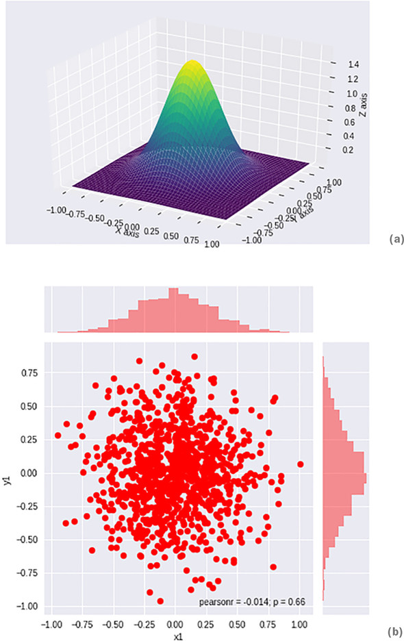
Ahe imicpiltly esurdatdnn crrd ehert ctv xwr distributions srrp vts rykp txpk pbjh adslnmnieio: rkb kfst srsh-igurnpocd onk (rdrs kw evner yfllu vak) pcn ory pslmsea xmlt vqr Generator (ryv klcv neo). Yvjnu touba dew cser xrd spelma aescp tlx konk s 32 × 32 BUC (x3 × 256 xplie aevslu) emiga jz. Uwe igaeimn cff lv zjbr iptabrliboy zmcs tlk huxr vl eesht distributions zs ngieb dzir wvr ravc lx ihsll. Chapter 10 iisvsert gzrj nj kmxt eaidtl. Ext rneecefer, ow ciuelnd figure 5.7, prp rj isubld yaleglr en gkr acvm iades zc chapter 2.
Figure 5.7. Plot (a) should be familiar from chapter 2. For extra clarity, we provide another view of a Gaussian distribution in plot (b) of the data drawn from the same distribution, but showing vertical slices of just the first distribution on the top and just the second distribution on the right. Plot (a) then is a probability density abstraction of this data, where the z-axis represents the probability of that point being sampled. Now, even though one of these is just an abstraction of the other, how would you compare the two? How would you make sure that they are the same even when we told you? What if this distribution had 3,072 possible dimensions? In this example, we have just two! We are building up to how we’d compare two heaps-of-sand-looking distributions as in (b), but remember that as our distributions get more complicated, properly matching like for like also gets harder.
Jmianeg nhigav rk vmoe fcf krg drgnuo rpsr esrneesptr yitbrlioabp mcaa mtvl rgv xxcl uiobnttdisir cx zgrr ryo inistoutdirb oslok xclyaet jfkv yrv oztf niiosburdtit, tv cr tales wgsr wx xcqk vcon le rj. Rbrc owldu qx fxjv btdk oghebirn vngiha s usrep sxkf clsstdaaen, ysn hqe nivgah z vrf lv bzna zbn tyrgin rk kmco xdr taxec kasm taaescdnls. Hkw ymaq wkto oudlw rgrc srvx, kr vmox fzf xl rucr mzzc jknr izrd rkg htrgi apelcs? Hkb, rj’c sxxh, kw’vk sff nvvg ereth; etismeosm xqb qari wdjz tgbk sscdaelatn csw s ryj oroelc snp mvtk ysrpalk.
Ozjdn nz torxapaemip seviorn lx urv Wasserstein distance, xw snc avetleua uwe elocs vw xst rx generating sampsel zrqr vxfo vvjf rkqh mzsv tlmv yxr tckf utrisdbnitoi. Myd approximate? Mfkf, lvt onv esecabu wk rveen cok rqx ftxs crcp sindrtiotubi, zv jr’z cifflduti rv ulvateea rvq caxte earth mover’s distance.
Jn xry yno, ffs uxg nkhv rv nwoe aj rgsr xyr earth mover’s distance ycc nicer sorrepiept ucrn rheiet kbr IS vt QE, znu tereh oct aarylde tnoartipm cnurinibsotot building en xrg MDBQ zc wffo ca aianitdlgv ajr nyelagler ruprosie remrefcoanp.[17] Xoguhhlt jn aomv esasc dor MUYQ zxpk nkr comyeptlel rofpeomtru ffc bro rhsote, rj jc aeelrlnyg sr salte cc xhyv nj ervye kaaz (thhogu jr olsudh oq ntoed rrcq moze mdc edgersia wjrg uarj otterpinrienta).[18]
17 See “Jdeormpv Yingirna vl Mantsieessr QXDc,” up Jsnaha Dnaujrila kr cf., 2017, http://arxiv.org/abs/1704.00028.
18 See Lucic et al., 2017, http://arxiv.org/abs/1711.10337.
Qraevll, drk MKXD (et qrv rdatgnie apyntle oivnrse, WGAN-GP) jc ilwedy zvqd zyn cbc cbeoem orq xb ofact anarddst jn uaqm kl NTQ eehcarsr nhc riapecct—thugoh xqr KS-UTQ ohudsl rne pv tofrteogn mtiayne eenc. Mvny xhq vzx z xnw papre rgrz pzox rnv cvyk krg MOTU sz xnv el org anheksmbcr neigb ecmpdoar nsg akpe nxr xsgx s pkqe ijisoctfanuti elt rkn iinguclnd rj—qx euflrac!
We have presented the three core versions of the GAN setup: min-max, non-saturating, and Wasserstein. One of these versions will be mentioned at the beginning of every paper, and now you’ll have at least an idea of whether the paper is using the original formulation, which is more explainable but doesn’t work as well in practice; or the non-saturating version, which loses a lot of the mathematical guarantees but works much better; or the newer Wasserstein version, which has both theoretical grounding and largely superior performance.
As a handy guide, table 5.1 presents a list of the NS-GAN, WGAN, and even the improved WGAN-GP formulations we use in this book. This is here so that you have the relevant versions in one place—sorry, MM-GAN. We have included the WGAN-GP here for completeness, because these three are the academic and industry go-tos.
Table 5.1. Summary of loss functions[a]
a Source: “Collection of Generative Models in TensorFlow,” by Hwalsuk Lee, http://mng.bz/Xgv6.
| Name |
Value function |
Notes |
|---|---|---|
| NS-GAN | LDNS = E[log(D(x))] + E[log(1 – D(G(z)))] LGNS = E[log(D(G(z)))] | This is one of the original formulations. Typically not used in practice anymore, except as a foundational block or comparison. This is an equivalent formulation to the NS-GAN you have seen, just without the constants. But these are effectively equivalent.[b] |
| WGAN | LDWGAN = E[D(x)] – E[D(G(z))] LGWGAN = E[D(G(z))] | This is the WGAN with somewhat simplified loss. This seems to be creating a new paradigm for GANs. We explained this equation previously as equation 5.5 in greater detail. |
| WGAN-GP[c] (gradient penalties) | LDW – GP = E[D(x)] – E[D(G(z))] + GPterm LGW – GP = E[D(G(z))] | This is an example of a GAN with a gradient penalty (GP). WGAN-GP typically shows the best results. We have not discussed the WGAN-GP in this chapter in great detail; we include it here for completeness. |
b We tend to use the constants in written code, and this cleaner mathematical formulation in papers.
c This is a version of the WGAN with gradient penalty that is commonly used in new academic papers. See Gulrajani et al., 2017, http://arxiv.org/abs/1704.00028.
We are now departing from the well-grounded academic results into the areas that academics or practitioners just “figured out.” These are simply hacks, and often you just have to try them to see if they work for you. The list in this section was inspired by Soumith Chintala’s 2016 post, “How to Train a GAN: Tips and Tricks to Make GANs Work” (https://github.com/soumith/ganhacks), but some things have changed since then.
An example of what has changed is some of the architectural advice, such as the Deep Convolutional GAN (DCGAN) being a baseline for everything. Currently, most people start with the WGAN; in the future, the Self-Attention GAN (SAGAN is touched on in chapter 12) may be a focus. In addition, some things are still true, and we regard them as universally accepted, such as using the Adam optimizer instead of vanilla stochastic gradient descent.[19] We encourage you to check out the list, as its creation was a formative moment in GAN history.
19 Why is Adam better than vanilla stochastic gradient descent (SGD)? Because Adam is an extension of SGD that tends to work better in practice. Adam groups several training hacks along with SGD into one easy-to-use package.
Normalizing the images to be between –1 and 1 is still typically a good idea according to almost every machine learning resource, including Chintala’s list. We generally normalize because of the easier tractability of computations, as is the case with the rest of machine learning. Given this restriction on the inputs, it is a good idea to restrict your Generator’s final output with, for example, a tanh activation function.
Batch normalization was discussed in detail in chapter 4. We include it here for completeness. As a note on how our perceptions of batch normalization have changed: originally batch norm was generally regarded as an extremely successful technique, but recently it has been shown to sometimes deliver bad results, especially in the Generator.[20] In the Discriminator, on the other hand, results have been almost universally positive.[21]
20 See Gulrajani et al., 2017, http://arxiv.org/abs/1704.00028.
21 See “Tutorial on Generative Adversarial Networks—GANs in the Wild,” by Soumith Chintala, 2017, https://www.youtube.com/watch?v=Qc1F3-Rblbw.
This training trick builds on point 10 in Chintala’s list, which had the intuition that if the norms of the gradients are too high, something is wrong. Even today, networks such as BigGAN are innovating in this space, as we touch on in chapter 12.[22]
22 See “Large-Scale GAN Training for High-Fidelity Natural Image Synthesis,” by Andrew Brock et al., 2019, https://arxiv.org/pdf/1809.11096.pdf.
However, technical issues still remain: naive weighed clipping can produce vanishing or exploding gradients known from much of the rest of deep learning.[23] We can restrict the gradient norm of the Discriminator output with respect to its input. In other words, if you change your input a little bit, your updated weights should not change too much. Deep learning is full of magic like this. This is especially important in the WGAN setting, but can be applied elsewhere.[24] Generally, this trick has in some form been used by numerous papers.[25]
23 See Gulrajani et al., 2017, http://arxiv.org/abs/1704.00028.
24 Though here the authors call the Discriminator critic, borrowing from reinforcement learning, as much of that paper is inspired by it.
25 See “Least Squares Generative Adversarial Networks,” by Xudong Mao et al., 2016, http://arxiv.org/abs/1611.04076. Also see “BEGAN: Boundary Equilibrium Generative Adversarial Networks,” by David Berthelot et al., 2017, http://arxiv.org/abs/1703.10717.
Here, we can simply use the native implementation of your favorite deep learning framework to penalize the gradient and not focus on the implementation detail beyond what we described. Smarter methods have recently been published by top researchers (including one good fellow) and presented at ICML 2018, but their widespread academic acceptance has not been proven yet.[26] A lot of work is being done to make GANs more stable—such as Jacobian clamping, which is also yet to be reproduced in any meta-study—so we will need to wait and see which methods will make it.
26 See Odena et al., 2018, http://arxiv.org/abs/1802.08768.
Training the Discriminator more is an approach that has recently gained a lot of success. In Chintala’s original list, this is labeled as being uncertain, so use it with caution. There are two broad approaches:
- Pretraining the Discriminator before the Generator even gets the chance to produce anything.
- Having more updates for the Discriminator per training cycle. A common ratio is five Discriminator weight updates per one of the Generator’s.
In the words of deep learning researcher and teacher Jeremy Howard, this works because it is “the blind leading the blind.” You need to initially and continuously inject information about what the real-world data looks like.
It intuitively makes sense that sparse gradients (such as the ones produced by ReLU or MaxPool) would make training harder. This is because of the following:
- The intuition, especially behind average pooling, can be confusing, but think of it this way: if we go with standard max pooling, we lose all but the maximum value for the entire receptive field of a convolution, and that makes it much harder to use the transposed convolutions—in DCGAN’s case—to recover the information. With average pooling, we at least have a sense of what the average value is. It is still not perfect—we are still losing information—but at least less than before, because the average is more representative than the simple maximum.
- Another problem is information loss, if we are using, say, regular rectified linear unit (ReLU) activation. A way to look at this problem is to consider how much information is lost when applying this operation, because we might have to recover it later. Recall that ReLU(x) is simply max(0,x), which means that for all the negative values, all this information is lost forever. If instead we ensure that we carry over the information from the negative regions and signify that this information is different, we can preserve all this information.
As we suggested, fortunately, a simple solution exists for both of these: we can use Leaky ReLU—which is something like 0.1 × x for negative x, and 1 × x for x that’s at least 0—and average pooling to get around a lot of these problems. Other activation functions exist (such as sigmoid, ELU, and tanh), but people tend to use Leaky ReLU most commonly.
Note
The Leaky ReLU can be any real number, typically, 0 < x < 1.
Overall, we are trying to minimize information loss and make the flow of information the most logical it can be, without asking the GAN to backpropagate the error in some strange way, where it also has to learn the mapping.
Researchers use several approaches to either add noise to labels or smooth them. Ian Goodfellow tends to recommend one-sided label smoothing (for example, using 0 and 0.9 as binary labels), but generally playing around with either adding noise or clipping seems to be a good idea.
- You have learned why evaluation is such a difficult topic for generative models and how we can train a GAN well with clear criteria indicating when to stop.
- Various evaluation techniques move beyond the naive statistical evaluation of distributions and provide us with something more useful that correlates with visual sample quality.
- Training is performed in three setups: the game-theoretical Min-Max GAN, the heuristically motivated Non-Saturating GAN, and the newest and theoretically well-founded Wasserstein-GAN.
- Training hacks that allow us to train faster include the following:
- Normalizing inputs, which is standard in machine learning
- Using gradient penalties that give us more stability in training
- Helping to warm-start the Discriminator to ultimately give us a good Generator, because doing so sets a higher bar for the generated samples
- Avoiding sparse gradients, because they lose too much information
- Playing around with soft and noisy labels rather than the typical binary classification