This chapter covers
- Using labels to train both the Generator and the Discriminator
- Teaching GANs to generate examples matching a specified label
- Implementing a Conditional GAN (CGAN) to generate handwritten digits of our choice
In the previous chapter, you learned about the SGAN, which introduced you to the idea of using labels in GAN training. SGANs use labels to train the Discriminator into a powerful semi-supervised classifier. In this chapter, you’ll learn about the Conditional GAN (CGAN), which uses labels to train both the Generator and the Discriminator. Thanks to this innovation, a Conditional GAN allows us to direct the Generator to synthesize the kind of fake examples we want.
As you have seen throughout this book, GANs are capable of producing examples ranging from simple handwritten digits to photorealistic images of human faces. However, although we could control the domain of examples our GAN learned to emulate by our selection of the training dataset, we could not specify any of the characteristics of the data samples the GAN would generate. For instance, the DCGAN we implemented in chapter 4 could synthesize realistic-looking handwritten digits, but we could not control whether it would produce, say, the number 7 rather than the number 9 at any given time.
Gn smlpie datasets vvfj rpo WKJSX, jn which aeplexms nogble xr uknf kxn vl 10 ssaclse, rjga ccnroen umc xakm livrtia. Jl, tvl csnantie, kqt qvfc aj rk oeucprd vry mbruen 9, xw nzs cirg koxu generating eaesxmpl tunli xw oyr rxp reubmn wv nswr. Qn texm cmepoxl rzqc-egaetnnoir tkass, evewohr, bro noadim le oibslspe wesrsan rbxa xre grale etl baad s rbeut-ecofr nlsootiu xr px taiclprac. Aovz, etl lpeamxe, ykr zzvr lx generating uhman eacsf. Ta svmreipesi cc rux gemias dpduocre dh dkr Lgeoisrsevr UTK eltm chapter 6 xzt, vw kpxc xn oltrcno ektx zdrw xsls fjfw pvr croedpdu. Ctpkk jc nv sdw kr rctdei qkr Generator rv eihynztsse, dcs, s mfvc et s afmlee clzx, rxf elnao trhoe tseeuarf csby cs cbv tv ciflaa opresnisxe.
Yvp byiailt xr edcedi swqr nuoj kl ssbr jfwf od edeergtan senpo xyr xthv vr z zzxr arayr lx iaapticpolns. Cc z osmwhaet tdiernvco aeemlpx, inmeiag rsdr wx oct etedviscte gloivsn c rmeurd ymtsyre, nqs s tnsiwes ceidrebss vpr reilkl cz c lidemd-qzkb nwmao rjpw fxqn xtg djzt nuz eerng zobv. Jr owdlu talyrge deeixtep obr cepsros lj distnae vl rihing c sketch tstira (kdw snz cdoerup fune nkk ksecht sr s mrjv), wk ldcou neetr bvr svderepitic euseratf njxr c cumotpre mrgpoar nbz vyxz rj ottpuu s eagnr lv afces gthcianm odr eitaircr. Kqt eiwstns oprn luodc opnti ad re yrx vne zrgr elseebrms kpr rinclmai rvma ecsolly.
Mo tvc pcxt hxb asn knith vl nchm orteh ccilarpat iancpailptos lvt hchiw qrx aiibylt rv ngreetea nc aiemg rusr seatchm kry ictraeir lv tkq ieccho uwdol oq c bcvm-engarch. Jn adilmec hceerars, wx cuold geidu yrk itoanerc kl vwn tghg oundmposc; jn lmkiifagmn nhc computer-generated imagery (CGI), ow oludc rtecea yrx txeac nseec ow zrwn rwjq immnial unpti tmxl munah stamnoira. Cod ajfr xyav nk.
Cdv YNXU aj nox xl vrq rtifs OTD viotisnonan srrb sukm targeted data rnaegieotn obspleis, unc lubyarag oyr rmce lflainuitne vne. Jn kry drieaenrm le rzju hepctra, xhb jwff lerna ewq TUTGa ovtw zbn temielnmp c lslam-ascel ironesv uy using (pqe esugsde jr!) rpv MNIST dataset.
Jcndrdetuo nj 2014 dd Orineyivst lv Wrtlaeno LdU snutted Whjdv Wajct shn Plrkic TJ hecittarc Snmkj Gsneidro, Conditional GAN zj z ntaregieve lsraaevdira nerwtok whseo Generator hzn Discriminator xzt tceoddnoini dgriun training yq using amvx oialandtid imofontanir.[1] Cjzb xuaiaylri nnrfomaoiti oulcd og, jn heyrot, nhtigany, paau cz s lssca blael, z arv le zcbr, tx nkxo c rinttwe tisedinpcor. Zkt talyicr nzy mlitpsycii, wo wffj ozh labels ac uro giocntiodnni roanmitfoni zz kw lxpanei dew RNYK okrws.
1 See “Xitoldnoani Dtvaneeire Revrslaidar Ukra,” qg Wpjyx Wtscj nps Smjxn Dndoiers, 2014, https://arxiv.org/abs/1411.1784.
Ugrnui YNRU training, drk Generator nraesl kr odupcre ireactsil semplxae ltx ouzs lblae nj rxp training attased, nzb roy Discriminator seanrl rk gssuitdiinh ools eaxepml-lleba ipras mxtl tfxc mexapel-llbea sirpa. Jn trtaonsc vr vry Svjm-Sespuidevr UCQ lmkt rgv esiuvpor htercpa, wsohe Discriminator nrseal xr iansgs rpv tcocrer alble er szod fxst xemlpae (nj datndiio rv higunsgtiiinsd tfsk maxselpe xtlm volz kavn), drk Discriminator jn c AKRG kvyc xnr rlaen er dtnieiyf chhiw sacls ja ichhw. Jr laerns nufx er epacct tfvc, tinhgmca rsiap liehw rjngietec asirp brzr ctx dchstiemam qns apirs jn ihchw brv amlepxe zj leck.
Vkt meeaplx, dxr XOXK Discriminator hodusl laenr xr jeterc qvr jtzh (![]() , 4), ersagedrls xl herwhte rxq epxalem (idwnntrtahe mrlenua 3) jc fsvt vt klxs, cabeseu rj xcqo nxr htmca xur leabl, 4. Axp BDTO Discriminator lshodu fcze alnre er jtcere fcf iameg-lebal psira jn cihwh ryk eigma jz kecl, enok lj rky lblea ateshmc grv mgeia.
, 4), ersagedrls xl herwhte rxq epxalem (idwnntrtahe mrlenua 3) jc fsvt vt klxs, cabeseu rj xcqo nxr htmca xur leabl, 4. Axp BDTO Discriminator lshodu fcze alnre er jtcere fcf iameg-lebal psira jn cihwh ryk eigma jz kecl, enok lj rky lblea ateshmc grv mgeia.
Ycnlrgdocyi, nj drero kr lvvf rop Discriminator, rj aj rnx gnoheu ktl rkd ANBO Generator rv peuocdr itslcarie-ogoknli zzrg. Ybx slmpeaxe jr aetgeresn asfe yxvn xr mathc hrtie labels. Rlrtx our Generator ja ylflu itdanre, zrqj qrno lsolaw ad kr cyspief wrcq eexlpma wo crnw rvq RQXK rk hzneitessy pu anpssig jr qrx erisded lblea.
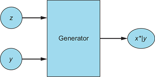
Rv lozarefmi nhitsg z jyr, rvf’a zfsf vpr cionitdngnio lbale y. Ckd Generator xccd dxr noise tcervo z cny vyr alleb y xr ienzstyshe s zkol xleeamp G(z, y) = x*|y (tgso cz “x* ivgne rsdr, tx idionctedon nv, y”). Rpk yfvs vl rqzj xlxs pameelx jz re kxfe (jn qor zpkk lv bvr Discriminator) cs elsoc za seilsobp vr s tfsk emplaxe lte dxr egvni elalb. Figure 8.1 uerasllistt rvu Generator.
Figure 8.1. CGAN Generator: G(z, y) = x*|y. Using random noise vector z and label y as inputs, the Generator produces a fake example x*|y that strives to be a realistic-looking match for the label.
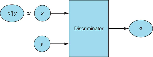
Avq Discriminator iecrvsee tfsx saexepml wjbr labels (x, y), chn lxzo expmelsa jbrw dxr laelb avug er ergaetne rqkm, (x*|y, y). Gn krg tfoc eealmpx-alble irpas, vrg Discriminator lneasr qwv er cnreeogiz tofs rcsq and pwx rk oirezgnce gmcithan ripas. Nn qxr Generator-oderpudc ealspxem, jr rnasel vr geroenciz lkxs egami-eblal irsap, htebrye nrealign kr ffrv mrku atpar tkml gkr sfxt nkec.
Yvd Discriminator tpsouut c ngeisl lbtryipaibo naiiigtdcn zrj convcotiin srrb rqx tnuip zj c ftxs, thicmang jtuz. Cgk Discriminator ’z zvfd jz er nearl xr tcjeer ffs clvk aexspelm yzn sff esmpxale gcrr ljfc rx hcmat tiher alebl, leiwh ctcgianpe fsf xtfs ealpmxe-alleb psira, sc wnhso nj figure 8.2.
Figure 8.2. The CGAN Discriminator receives real examples along with their labels (x, y) and fake examples along with the label used to synthesize them (x*|y, y). The Discriminator then outputs a probability (computed by the sigmoid activation function σ) indicating whether the input pair is real rather than fake.
The two CGAN subnetworks, their inputs, outputs, and objectives are summarized in table 8.1.
Table 8.1. CGAN Generator and Discriminator networks (view table figure)
| Generator |
Discriminator |
|
|---|---|---|
| Input | A vector of random numbers and a label: (z, y) | The Discriminator receives the following inputs:
|
| Output | Fake examples that strive to be as convincing as possible in matches for their labels: G(z, y) = x*|y | A single probability indicating whether the input example is a real, matching example-label pair |
| Goal | Generate realistic-looking fake data that match their labels | Distinguish between fake example-label pairs coming from the Generator and real example-label pairs coming from the training dataset |
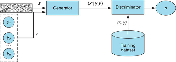
Putting it all together, figure 8.3 shows a high-level architecture diagram of a CGAN. Notice that for each fake example, the same label y is passed to both the Generator and the Discriminator. Also, note that the Discriminator is never explicitly trained to reject mismatched pairs by being trained on real examples with mismatching labels; its ability to identify mismatched pairs is a by-product of being trained to accept only real matching pairs.
Figure 8.3. The CGAN Generator uses a random noise vector z and a label y (one of the n possible labels) as inputs and produces a fake example x*|y that strives to be both realistic looking and a convincing match for the label y.
Note
You may have noticed a pattern: for almost every GAN variant, we present you with a table summarizing the inputs, outputs, and objectives of the Discriminator and Generator networks, and with a network architecture diagram. This is not by accident; indeed, one of the main goals of these chapters is to give you a mental template—a reusable framework of sorts—for the kind of things to look for when you encounter GAN implementations that diverge from the original GAN. Analyzing the Generator and Discriminator networks and the overall model architecture are often the best first steps.
The CGAN Discriminator receives fake labeled examples (x*|y, y) produced by the Generator and real labeled examples (x, y), and it learns to tell whether a given example-label is real or fake.
Enough for theory. It’s time we put what you have learned into practice and implement our own CGAN model.
In this tutorial, we will implement a CGAN model that learns to generate handwritten digits of our choice. At the end, we will generate a sample of images for each numeral to see how well the model learned to generate targeted data.
Our implementation is inspired by the CGAN in the open source GitHub repository of GAN models in Keras (the same one we used in chapters 3 and 4).[2] In particular, we use the repository’s approach of using Embedding layers to combine examples and labels into joint hidden representations (more on this later).
2 See Erik Linder-Norén’s Keras-GAN GitHub repository, 2017, https://github.com/eriklindernoren/Keras-GAN.
The rest of our CGAN model, however, diverges from the one found in the Keras-GAN repository. We refactored the embedding implementation to be more readable and added detailed explanatory comments. Crucially, we also adapted our CGAN to use convolutional neural networks, which yield significantly more realistic examples—recall the difference between the images produced by the GAN in chapter 3 and the DCGAN in chapter 4!
A Jupyter notebook with the full implementation, including added visualizations of the training progress, is available in our GitHub repository, under the chapter-8 folder: https://github.com/GANs-in-Action/gans-in-action. The code was tested with Python 3.6.0, Keras 2.1.6, and TensorFlow 1.8.0. To speed up the training time, we recommend running the model on a GPU.
You guessed it—the first step is to import all the modules and libraries needed for our model, as shown in the following listing.
Listing 8.1. Import statements
%matplotlib inline

import matplotlib.pyplot as plt
import numpy as np

from keras.datasets import mnist
from keras.layers import (
        Activation, BatchNormalization, Concatenate, Dense,
        Embedding, Flatten, Input, Multiply, Reshape)
from keras.layers.advanced_activations import LeakyReLU
from keras.layers.convolutional import Conv2D, Conv2DTranspose
from keras.models import Model, Sequential
from keras.optimizers import Adam
Just as before, we also specify the input image size, the size of the noise vector z, and the number of classes in our dataset, as shown here.
Listing 8.2. Model input dimensions
img_rows = 28
img_cols = 28
channels = 1

img_shape = (img_rows, img_cols, channels)     #1

z_dim = 100                                    #2

num_classes = 10                               #3
In this section, we implement the CGAN Generator. By now, you should be familiar with much of this network from chapters 4 and 7. The modifications made for the CGAN center around input handling, where we use embedding and element-wise multiplication to combine the random noise vector z and the label y into a joint representation. Let’s walk through what the code does:
- Take label y (an integer from 0 to 9) and turn it into a dense vector of size z_dim (the length of the random noise vector) by using the Keras Embedding layer.
- Combine the label embedding with the noise vector z into a joint representation by using the Keras Multiply layer. As its name suggests, this layer multiplies the corresponding entries of the two equal-length vectors and outputs a single vector of the resulting products.
- Feed the resulting vector as input into the rest of the CGAN Generator network to synthesize an image.
Figure 8.4 illustrates the process, using the label 7 as an example.
Figure 8.4. The steps used to combine the conditioning label (7 in this example) and the random noise vector z into a single joint representation
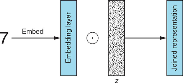
First, we embed the label into a vector of the same size as z. Second, we multiply the corresponding elements of the embedded label and z (the symbol denotes element-wise multiplication). The resulting joined representation is then used as input into the CGAN Generator network.
And finally, the following listing shows what it all looks like in Python/Keras code.
Listing 8.3. CGAN Generator
def build_generator(z_dim):

    model = Sequential()

    model.add(Dense(256 * 7 * 7, input_dim=z_dim))                           #1
    model.add(Reshape((7, 7, 256)))

    model.add(Conv2DTranspose(128, kernel_size=3, strides=2, padding='same'))#2

    model.add(BatchNormalization())                                          #3

    model.add(LeakyReLU(alpha=0.01))                                         #4

    model.add(Conv2DTranspose(64, kernel_size=3, strides=1, padding='same')) #5

    model.add(BatchNormalization())                                          #3

    model.add(LeakyReLU(alpha=0.01))                                         #4

    model.add(Conv2DTranspose(1, kernel_size=3, strides=2, padding='same'))  #6

    model.add(Activation('tanh'))                                            #7

    return model


def build_cgan_generator(z_dim):

    z = Input(shape=(z_dim, ))                                               #8

    label = Input(shape=(1, ), dtype='int32')                                #9

    label_embedding = Embedding(num_classes, z_dim, input_length=1)(label)   #10

    label_embedding = Flatten()(label_embedding)                             #11

    joined_representation = Multiply()([z, label_embedding])                 #12

    generator = build_generator(z_dim)

    conditioned_img = generator(joined_representation)                       #13

    return Model([z, label], conditioned_img)
Next, we implement the CGAN Discriminator. Just as in the previous section, the network architecture should look familiar to you, except for the piece where we handle the input image and its label. Here, too, we use the Keras Embedding layer to turn input labels into dense vectors. However, unlike the Generator, where the model input is a flat vector, the Discriminator receives three-dimensional images. This necessitates customized handling, described in the following steps:
- Take a label (an integer from 0 to 9) and—using the Keras Embedding layer—turn the label into a dense vector of size 28 × 28 × 1 = 784 (the length of a flattened image).
- Reshape the label embeddings into the image dimensions (28 × 28 × 1).
- Concatenate the reshaped label embedding onto the corresponding image, creating a joint representation with the shape (28 × 28 × 2). You can think of it as an image with its embedded label “stamped” on top of it.
- Feed the image-label joint representation as input into the CGAN Discriminator network. Note that in order for things to work, we have to adjust the model input dimensions to (28 × 28 × 2) to reflect the new input shape.
Again, to make it less abstract, let’s see what the process looks like visually, using the label 7 as an example; see figure 8.5.
Figure 8.5. The steps used to combine the label (7 in this case) and the input image into a single joint representation
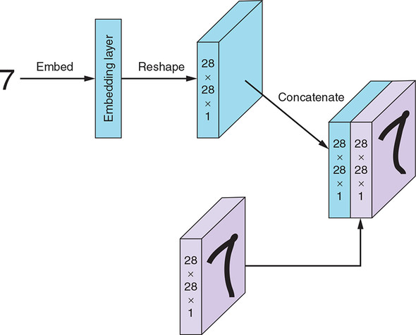
First, we embed the label into a vector the size of a flattened image (28 × 28 × 1 = 784). Second, we reshape the embedded label into a tensor with the same shape as the input image (28 × 28 × 1). Third, we concatenate the reshaped label that is embedding onto the corresponding image. This joined representation is then passed as input into the CGAN Discriminator network.
In addition to the preprocessing steps, we have to make a few additional adjustments to the Discriminator network compared to the one in chapter 4. (As in the previous chapter, basing the model on our DCGAN implementation should make it easier to see the CGAN-specific changes without distractions from implementation details in unrelated parts of the model.) First, we have to adjust the model input dimensions to (28 × 28 × 2) to reflect the new input shape.
Second, we increase the depth of the first convolutional layer from 32 to 64. The reasoning behind this change is that there is more information to encode because of the concatenated label embedding; this network architecture indeed yielded better results experimentally.
At the output layer, we use the sigmoid activation function to produce a probability that the input image-label pair is real rather than fake—no change here. And finally, the following listing is our CGAN Discriminator implementation.
Listing 8.4. CGAN Discriminator
def build_discriminator(img_shape):

    model = Sequential()

    model.add(                                                        #1

        Conv2D(64,
               kernel_size=3,
               strides=2,
               input_shape=(img_shape[0], img_shape[1], img_shape[2] + 1),
               padding='same'))

    model.add(LeakyReLU(alpha=0.01))                                  #2

    model.add(                                                        #3
        Conv2D(64,
               kernel_size=3,
               strides=2,
               input_shape=img_shape,
               padding='same'))

    model.add(BatchNormalization())                                   #4

    model.add(LeakyReLU(alpha=0.01))                                  #5

    model.add(                                                        #6
        Conv2D(128,
               kernel_size=3,
               strides=2,
               input_shape=img_shape,
               padding='same'))

    model.add(BatchNormalization())                                   #7

    model.add(LeakyReLU(alpha=0.01))                                  #8

    model.add(Flatten())                                              #9
    model.add(Dense(1, activation='sigmoid'))

    return model


def build_cgan_discriminator(img_shape):

    img = Input(shape=img_shape)                                      #10

    label = Input(shape=(1, ), dtype='int32')                         #11

    label_embedding = Embedding(num_classes,                          #12
                                np.prod(img_shape),
                                input_length=1)(label)

    label_embedding = Flatten()(label_embedding)                      #13

    label_embedding = Reshape(img_shape)(label_embedding)             #14

    concatenated = Concatenate(axis=-1)([img, label_embedding])       #15

    discriminator = build_discriminator(img_shape)

    classification = discriminator(concatenated)                      #16

    return Model([img, label], classification)
Next, we build and compile the CGAN Discriminator and Generator models, as shown in the following listing. Notice that in the combined model used to train the Generator, the same input label is passed to the Generator (to generate a sample) and to the Discriminator (to make a prediction).
Listing 8.5. Building and compiling the CGAN model
def build_cgan(generator, discriminator):

    z = Input(shape=(z_dim, ))                               #1

    label = Input(shape=(1, ))                               #2

    img = generator([z, label])                              #3

    classification = discriminator([img, label])

    model = Model([z, label], classification)                #4

    return model


discriminator = build_cgan_discriminator(img_shape)          #5
discriminator.compile(loss='binary_crossentropy',
                      optimizer=Adam(),
                      metrics=['accuracy'])

generator = build_cgan_generator(z_dim)                      #6

discriminator.trainable = False                              #7

cgan = build_cgan(generator, discriminator)                  #8
cgan.compile(loss='binary_crossentropy', optimizer=Adam())
CGAN training algorithm
For each training iteration do
- Train the Discriminator:
- Take a random mini-batch of real examples and their labels (x, y).
- Compute D((x, y)) for the mini-batch and backpropagate the binary classification loss to update θ(D) to minimize the loss.
- Take a mini-batch of random noise vectors and class labels (z, y) and generate a mini-batch of fake examples: G(z, y) = x*|y.
- Compute D(x*|y, y) for the mini-batch and backpropagate the binary classification loss to update θ(D) to minimize the loss.
- Train the Generator:
- Take a mini-batch of random noise vectors and class labels (z, y) and generate a mini-batch of fake examples: G(z, y) = x*|y.
- Compute D(x*|y, y) for the given mini-batch and backpropagate the binary classification loss to update θ(G) to maximize the loss.
End for
The following listing implements this CGAN training algorithm.
Listing 8.6. CGAN training loop
accuracies = []
losses = []


def train(iterations, batch_size, sample_interval):

    (X_train, y_train), (_, _) = mnist.load_data()                           #1

    X_train = X_train / 127.5 - 1.                                           #2
    X_train = np.expand_dims(X_train, axis=3)

    real = np.ones((batch_size, 1))                                          #3

    fake = np.zeros((batch_size, 1))                                         #4

    for iteration in range(iterations):


        idx = np.random.randint(0, X_train.shape[0], batch_size)             #5
        imgs, labels = X_train[idx], y_train[idx]

        z = np.random.normal(0, 1, (batch_size, z_dim))                      #6
        gen_imgs = generator.predict([z, labels])

        d_loss_real = discriminator.train_on_batch([imgs, labels], real)     #7
        d_loss_fake = discriminator.train_on_batch([gen_imgs, labels], fake)
        d_loss = 0.5 * np.add(d_loss_real, d_loss_fake)

        z = np.random.normal(0, 1, (batch_size, z_dim))                      #8

        labels = np.random.randint(0, num_classes, batch_size).reshape(-1, 1)#9

        g_loss = cgan.train_on_batch([z, labels], real)                      #10

        if (iteration + 1) % sample_interval == 0:

            print("%d [D loss: %f, acc.: %.2f%%] [G loss: %f]" %             #11
                  (iteration + 1, d_loss[0], 100 * d_loss[1], g_loss))

            losses.append((d_loss[0], g_loss))                               #12
            accuracies.append(100 * d_loss[1])

            sample_images()                                                  #13
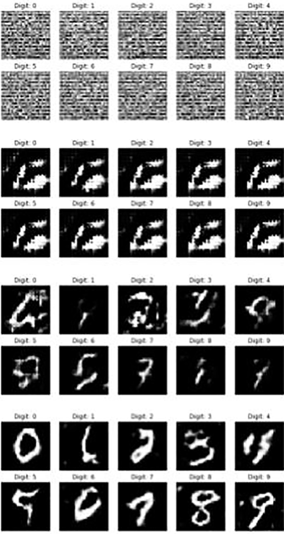
You may recognize the next function from chapters 3 and 4. We used it to examine how the quality of the Generator-produced images improved as the training progressed. The function in listing 8.7 is indeed similar, but a few crucial differences exist.
First, instead of a 4 × 4 grid of random handwritten digits, we are generating a 2 × 5 grid of numbers, 1 through 5 in the first row, and 6 through 9 in the second row. This allows us to inspect how well the CGAN Generator is learning to produce specific numerals. Second, we are displaying the label for each example by using the set_title() method.
Listing 8.7. Displaying generated images
def sample_images(image_grid_rows=2, image_grid_columns=5):

    z = np.random.normal(0, 1, (image_grid_rows * image_grid_columns, z_dim))#1

    labels = np.arange(0, 10).reshape(-1, 1)                                 #2

    gen_imgs = generator.predict([z, labels])                                #3

    gen_imgs = 0.5 * gen_imgs + 0.5                                          #4

    fig, axs = plt.subplots(image_grid_rows,                                 #5
                            image_grid_columns,
                            figsize=(10, 4),
                            sharey=True,
                            sharex=True)

    cnt = 0
    for i in range(image_grid_rows):
        for j in range(image_grid_columns):
            axs[i, j].imshow(gen_imgs[cnt, :, :, 0], cmap='gray')            #6
            axs[i, j].axis('off')
            axs[i, j].set_title("Digit: %d" % labels[cnt])
            cnt += 1
Figure 8.6 shows sample output from this function and illustrates the improvement to the CGAN-produced numerals over the course of training.
Figure 8.6. Starting from random noise, GCAN learns to produce realistic-looking numerals for each of the labels in the training dataset.
And finally, let’s run the model we just implemented:
iterations = 12000                                #1
batch_size = 32
sample_interval = 1000

train(iterations, batch_size, sample_interval)    #2
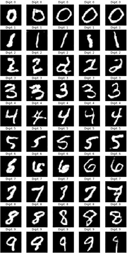
Figure 8.7 shows the images of digits produced by the CGAN Generator after it is fully trained. At each row, we instruct the Generator to synthesize a different numeral, from 0 to 9. Notice that each numeral is rendered in a different writing style, attesting to CGAN’s ability not only to learn to produce examples matching every label in the training dataset, but also to capture the full diversity of the training data.
Figure 8.7. Each row shows a sample of images produced to match a given numeral, 0 through 9. As you can see, the CGAN Generator has successfully learned to produce every class represented in our dataset.
In this chapter, you saw how labels could be used to guide the training of the Generator and the Discriminator to teach a GAN to produce fake examples of our choice. Along with the DCGAN, CGAN is one of the most influential early GAN variants that has inspired countless new research directions.
Perhaps the most impactful and promising of these is the use of conditional adversarial networks as a general-purpose solution to image-to-image translation problems. This is a class of problems that seeks to translate images from one modality into another. Applications of image-to-image translation range from colorizing black-and-white photos to turning a daytime scene into nighttime and synthesizing a satellite view from a map view.
One of the most successful early implementations based on the Conditional GAN paradigm is pix2pix, which uses pairs of images (one as the input and the other as the label) to learn to translate from one domain into another. Recall that, in theory as well as in practice, the conditioning information used to train a CGAN can be much more than just labels to provide for more complex use cases and scenarios. For example, for colorization tasks, an image pair would be a black-and-white photo (the input) and a colored version of the same photo (the label). You will see these illustrated in the following chapter.
We do not cover pix2pix in detail because only about a year after its publication, it was eclipsed by another GAN variant that not only outperformed pix2pix’s performance on image-to-image translation tasks but also accomplished it without the need for paired images. The Cycle-Consistent Adversarial Network (or CycleGAN, as the technique came to be known) needs only two groups of images representing the two domains (for example, a group of black-and-white photos and a group of colored photos). You will learn all about this remarkable GAN variant in the following chapter.
- Conditional GAN (CGAN) is a GAN variant in which both the Generator and the Discriminator are conditioned on auxiliary data such as a class label during training.
- The additional information constrains the Generator to synthesize a certain type of output and the Discriminator to accept only real examples matching the given additional information.
- As a tutorial, we implemented a CGAN that generates realistic handwritten digits of our choice by using MNIST class labels as our conditioning information.
- Embedding maps an integer into a dense vector of the desired size. We used embedding to create a joint hidden representation from a random noise vector and a label (for CGAN Generator training) and from an input image and a label (for CGAN Discriminator training).