4 Big-O notation: A framework for measuring algorithm efficiency
In this chapter
- objectively comparing different algorithms
- using big-O notation to understand data structures
- the difference between worst-case, average, and amortized analysis
- a comparative analysis of binary and linear search
In chapter 3, we discussed how binary search seems faster than linear search, but we didn’t have the tools to explain why. In this chapter, we introduce an analysis technique that will change the way you work—and that’s an understatement. After reading this chapter, you’ll be able to distinguish between the high-level analysis of the performance of algorithms and data structures and the more concrete analysis of your code’s running time. This will help you choose the right data structure and avoid bottlenecks before you dive into implementing code. With a little upfront effort, this will save you a lot of time and pain.
How do we choose the best option?
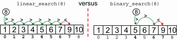
In chapter 3, you were introduced to two methods for searching a sorted array: linear and binary search. I told you that binary search is faster than linear, and you could see an example where binary search required only a few comparisons, while linear search had to scan almost the whole array instead.
You might think this was just a coincidence or I chose the example carefully to show you this result. Yes, of course, I totally did, but it turns out that this is also true in general, and only in edge cases, linear search is faster than binary.