This chapter covers
- Understanding the role of windows and the different types
- Handling out-of-order data
- Suppressing intermediate results
- Grokking the importance of timestamps
In previous chapters, you learned how to perform aggregations with KStream and KTable. This chapter will build on that knowledge and allow you to apply it to get more precise answers to problems involving aggregations. The tool you’ll use for this is windows. Using windows or windowing is putting aggregated data into discrete time buckets. This chapter teaches you how to apply windowing to your specific use cases.
Windowing is critical to apply because, otherwise, aggregations will continue to grow over time, and retrieving helpful information becomes difficult if all you have is a giant ball of facts without much context. As a high-level example, consider you’re responsible for staffing a pizza shop in the student union at your university (figure 9.1). The shop is open from 11 a.m. to 5 p.m. Total sales usually amount to 20 pizzas (this is your aggregation).
Figure 9.1 Just looking at a large aggregation doesn’t give the full picture.
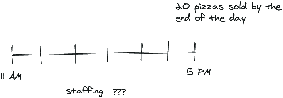
Determining how best to staff the shop is only possible with additional information, as you only know the total sold for the day. So you are left to guess that 20 pizzas over 6 hours amounts to roughly 3 pizzas per hour (figure 9.2), easily handled by two student workers, but is that the best choice?