3 Classifiers and vector calculus
We took a first look at the core concept of machine learning in section 1.3. Then, in section 2.8.2, we examined classifiers as a special case. But so far, we have skipped the topic of error minimization: given one or more training examples, how do we adjust the weights and biases to make the machine closer to the desired ideal? We will study this topic in this chapter by discussing the concept of gradients.
NOTE
The complete PyTorch code for this chapter is available at http://mng.bz /4Zya in the form of fully functional and executable Jupyter notebooks.
3.1 Geometrical view of image classification
To fix our ideas, consider a machine that classifies whether an image contains a car or a giraffe. Such classifiers, with only two classes, are known as binary classifiers. The first question is how to represent the input.
3.1.1 Input representation
The car-versus-giraffe scenario belongs to a special class of problems where we are analyzing a visual scene. Here, the inputs are the brightness levels of various points in the 3D scene projected onto a 2D image plane. Each element of the image represents a point in the actual scene and is referred to as a pixel. The image is a two-dimensional array representing the collection of pixel values at a given instant in time. It is usually scaled to a fixed size, say 224 × 224. As such, the image can be viewed as a matrix:
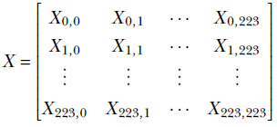
Each element of the matrix, Xi, j, is a pixel color value in the range [0,255].