3 Going on a random walk

In the previous chapter, we compared different naïve forecasting methods and we learned that they often serve as benchmarks for our more sophisticated models. However, there are instances where the simplest methods will yield the best forecasts. This is the case when we face a random walk process.

In this chapter, we will cover what a random walk process is, how to recognize it, and how to make forecasts using random walk models. Along the way, we will introduce the concepts of differencing, stationarity, and white noise that are used will come back in later chapters as we develop more advanced statistical learning models.

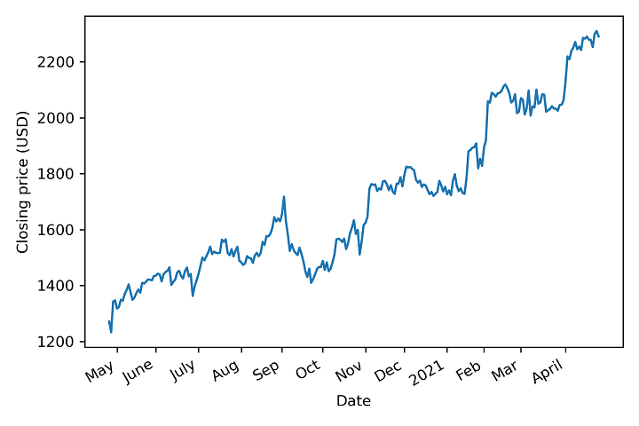
Suppose that you want to buy shares of Alphabet Inc. (GOOGL). Ideally, you would want to buy if the closing price of the stock is expected to go up in the future, otherwise, your investment will not be profitable. Hence, you decide to collect data on the daily closing price of GOOGL over one year and use time series forecasting to determine the future closing price of the stock. We can see the closing price of GOOGL between April 28, 2020, and April 27, 2021 in figure 3.1.

3.1 The random walk process

3.1.1 Simulating a random walk process

3.2 Identifying a random walk

3.2.1 Stationarity

3.2.2 Testing for stationarity

3.2.3 The autocorrelation function

3.2.4 Putting it all together

3.2.5 Is GOOGL a random walk?

3.3 Forecasting a random walk

3.3.1 Forecasting on a long horizon

3.3.2 Forecasting the next timestep

3.4 Exercises

3.4.1 Easy: simulate and forecast a random walk

3.4.2 Medium: Forecast the daily closing price of GOOGL

3.4.3 Hard: Forecast the daily closing price of a stock of your choice

3.5 Next steps

3.6  Summary