Chapter 2. Communication: basic input and output

An important part of any program is interacting with the user. For almost any program or game you might want to create, you’ll need to accept numbers, strings, or input from the user, display or draw output back to the user, or both. This chapter will teach you how to get strings and numbers from the user and write strings and numbers back.

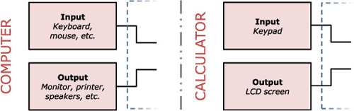
As you learned in chapter 1, your calculator shares its architecture with any common computer. You may recall that calculators and computers both have connected devices called input and output devices, as shown in figure 2.1. For computers, things like the monitor, the speakers, and the printer are the output. They’re devices the computer can instruct to communicate something to the user. Computers’ input devices, such as the keyboard, the mouse, and a microphone, let the user talk back to a computer. In much the same way, calculators have input and output devices for communication with the user: the keypad gives the user a way to instruct the calculator; the LCD screen lets the calculator show things back to the user.

In this chapter, you’ll be learning the rudiments of reading input from the keyboard and writing output back to the screen. In later chapters, you’ll learn more complex types of input and output, such as checking to see if specific keys were pressed or drawing a line on the screen. Imagine any simple math program, such as the quadratic solver that you created in chapter 1. It lets the user type in a few numbers, performs simple math on the values, and displays results to the user. In this chapter, you’ll learn to construct similar applications. You’ll write an animation, a program to raise a number to a power, and a program to calculate the slope of a line, among many others. You’ll even learn about accepting strings from the user, which will give you the skills to write a program to converse with your calculator. In the hope that you’ll start playing around with a few programs of your own as soon as possible, I’ll teach you the basics of troubleshooting errors or bugs in your programs.

The title of this chapter refers to “input and output,” a standard programming phrase, but you’ll learn how to output text and numbers to the screen first. If you learned input first, your program would be able to accept input from the user but wouldn’t be able to display anything back to the user to show that it had been able to do something useful with that input! Therefore, you’ll learn output first, so that when you learn input, you can output something based on the numbers or text the user just provided as input.

Before any of this, you need to meet the program editor and the homescreen, the pieces of your calculator’s built-in software that you’ll be using in this chapter.

2.1. Getting to know the program editor and homescreen

As someone who has used a graphing calculator to some extent for math and graphing, you should have the vague impression that there are different areas of the calculator’s built-in software, called its operating system, or OS. There’s the portion where you type math and get results, there’s the screen where you type equations to graph, and then there’s where you see your graphs drawn and can examine them. You may have even encountered menus such as the Statistics menu, the Window or Zoom menu, or the Memory menu. This and all the subsequent chapters will be largely spent in the program editor, where you type in the TI-BASIC source code for programs to run on your calculator.

We’ll begin with a look at the program editor, the section of your calculator’s OS you use to write software on the device itself. This section is about you, the programmer, typing source code into a program, which in a sense is input. But this isn’t the section on the input named in the chapter’s title; that input, where the user types data that your programs can then use, will be covered in section 2.3.

2.1.1. The program editor: typing source code

You first saw the Program menu and the program editor in chapter 1. You can access the Program menu by pressing the [PRGM] (program) key from the home-screen, the graph screen, or from almost anywhere else within the calculator’s OS. The Program menu holds three tabs labeled EXEC, EDIT, and NEW, as shown in figure 2.2.

You’ll find yourself using each of these three tabs often throughout the coming chapters; the function of each is summarized in table 2.1.

If you choose either to edit some existing program or create a program, you’ll find yourself within the program editor.

Inside the Program Editor

The program editor is the area you use to type in the source code for your program. It contains up to eight lines of text, which normally consist of one line showing the name of your program and seven lines of source code, as shown at the left side of figure 2.3. If your program is more than seven lines long, you can use the up- and down-arrow keys to move throughout the code.

As you type the programs in this and coming chapters into your calculator, and when you begin to make your own programs, you’ll spend a great deal of time inside the program editor. To use it effectively, you’ll need to know how exactly to type the different commands, letters, numbers, and symbols that make up the source code of any TI-BASIC program.

Understanding Keys and Their Functions

The program editor is similar to any text editor you may have used on a computer. You use the keys on the calculator’s keypad to type in numbers, letters, and symbols. As I explained in chapter 1, each key has up to three functions. When you press the key, you perform whatever function is printed directly on the key itself, which in some cases brings up a menu and in other cases types a token or a character. Table 2.2 shows how to access the (up to) three different functions for each key.

The keys and their functions are more or less the same throughout the entire calculator. You can use [2nd] and [ALPHA] the same way regardless of whether or not you’re in the program editor, so what do you need to know that’s specific to the program editor? You need to know where to find all of the commands used in programming.

Typing Commands into Programs

When you’re in the program editor, the meaning of the [PRGM] key changes and won’t show the set of three tabs, EXEC, EDIT, and NEW, that you see when you press the [PRGM] key from the homescreen. When you press [PRGM] from inside the program editor, it will instead show a different three-tab menu, the first two tabs of which, CTL and I/O, are displayed in figure 2.4. The EXEC tab contains a list of the programs on your calculator, which differs from calculator to calculator, so I don’t show you that tab. In section 4.4, I’ll show you how to use the contents of the EXEC tab.

You can scroll up and down each of the three tabs with the up- and down-arrow keys and move between the tabs using the left and right arrows. When you find the command you want, press [ENTER] to paste it into your program or press [CLEAR] to go back to the program editor without pasting any of the tokens. Table 2.3 explains what each tab is for.

Correcting Mistakes

Typing out programs line by line would be straightforward if humans were perfect, but we’re not. We need a way to correct our mistakes, to remove or add pieces to the program later, to insert text between existing text, and to create new lines or remove them. You might even find yourself wanting to paste the contents of one program into another. Luckily, the calculator’s program editor has easy ways to perform all of these tasks.

The [DEL] key will delete whatever is directly under the cursor, be it a token or a letter or symbol. You’ll notice that when you delete a token, the entire token is deleted at once, instead of letter by letter.

You can clear the contents of an entire line with [CLEAR], which you’ll probably soon learn the frustration of doing by accident.

On the flip side, you can insert text in the middle of lines. Press [2nd][DEL] to go into Insert mode: the cursor will change from a solid black box to an underscore. Now, when you type, the things you type will be inserted instead of replacing what was already there. You can insert new lines in the middle of your program by entering Insert mode and pressing [ENTER]. To leave Insert mode, press any of the arrow keys, and the cursor will change back to a black rectangle.

Copying Code

Now you’ll learn how to paste the contents of one program into another. It’s a trick used to rename a program: create a program with the new name, paste the contents of the program with the old name into the new program, and delete the old program from the calculator’s memory menu. You can also use it to prototype a piece of a program in a small program, test it out separately from the main program, then paste it into your program when you know it works without needing to type it out again. To paste a program into another program, follow these steps:

1.  Switch your editing mode from the normal Replace mode to Insert mode by pressing [2nd][DEL] (remember, [2nd] and then [DEL], not [2nd] and [DEL] together).

2.  Next, activate the Rcl (Recall) function by pressing [2nd][STO>].

3.  Press [PRGM], move to the [EXEC] tab, and choose the name of the program that you want to paste in.

4.  Hit [ENTER] to perform the Recall.

As well as adding code to programs and copying and pasting code between programs, you also occasionally need to delete old programs that you don’t need any more or that you merely created as an experiment.

Deleting a Program

Although it’s not strictly a task of the program editor, sooner or later you will want to know how to delete a program. After creating or editing programs, you may find your PRGM menu clogged with small test programs that you no longer need and that you’d like to clean off of your calculator. Deleting a program involves entering the Memory menu, which you may have encountered in your preprogramming use of your calculator:

1.  Quit to the homescreen if you’re not already there with [2nd][MODE].

2.  Press [2nd][+] to open the Memory menu, since the [+] key has MEM listed as its [2nd] function.

3.  Choose 2:Mem Mgmt/Del..., 7:Prgm...; move the arrow down to the program you want to delete and press [DEL].

4.  Once you confirm that you do indeed want to delete that program, the calculator will delete it.

Programs that have been deleted can’t be recovered, so make sure that you’re sure you don’t need a program any longer before you remove it. If your calculator is getting full, I recommend you back up old programs to your computer (see section A.6) before you delete them.

Don’t worry if you didn’t absorb all this information about using the program editor. As you type out the programs in this chapter and then start to write your own programs, you’ll swiftly become accustomed to using the editor. It’s intuitive, and even if you make errors, there’s little you can do to damage your calculator. As you work through the many programs presented in every chapter and write your own programs, you’ll spend a great deal of time inside the program editor, and you’ll gain proficiency in typing more quickly, remembering where to find each command, and moving around your code.

Now that you’ve learned the basics of using the program editor to type programs, I’ll introduce you to the homescreen. Just as the program editor is where you’ll create programs, the homescreen is the area where your program will interact with users as it runs by displaying output and accepting input.

2.1.2. The homescreen: your canvas for input and output

You already know the homescreen as the place where you do math and, if you’ve ever run programs on your calculator, as the place to where you paste programs’ names from the [PRGM] menu in order to run them. What you’ll learn in this chapter is how to display text and numbers on the homescreen and how to get the user to type in text and numbers for your program to use. The homescreen itself is an array of characters, 8 rows tall and 16 columns wide, as shown in figure 2.5. You can use it one line at a time, such as when you perform math calculations; you’ll also learn how to individually change each of the 128 spaces (16 * 8 = 128) in this chapter.

Clearing the Homescreen

It’s fine to display text, numbers, equations, and the like on the homescreen, but you’ll occasionally want to start with a clean slate. To remove everything on the home-screen, there’s a simple command called ClrHome. It will erase all 128 spaces in the homescreen and return the cursor to the top-left corner of the homescreen. If you then use functions to display text or ask for user input, those new contents will appear on this now-blank homescreen.

To demonstrate the effects of the ClrHome command, you can try the following program, CLRHOME. This may be the simplest TI-BASIC program you’ll ever try, containing a single command with no arguments. When you run this program, the only thing it will do is clear the contents of the homescreen. To enter this into your calculator, you need to know that the ClrHome command is under [PRGM][][8] or [PRGM][] 8:ClrHome.

Unfortunately, because every program ends by displaying “Done” on the homescreen, aligned at the right edge of the screen, the homescreen won’t be completely blank after you run this program. Figure 2.6 shows two screenshots, the first taken before the CLRHOME program is run, the second after.

You now know what the homescreen is, that you’ll be able to use it to communicate with the user in your programs, and how to clear it. The programs you will examine, write, and test in the remainder of this chapter, as well as chapters 3 and 4, will operate entirely on the homescreen, so you’ll continue to build your familiarity with it as you read on. Now you need to learn your first real set of calculator programming skills: displaying text on the homescreen.

2.2. Output: displaying text

Almost any program needs to display something back to the user to provide feedback on what’s happening inside the program. This might range from something as advanced as a graphical part of a game to something as simple as the numeric result of a calculation. I’ll start by teaching you the simpler end of the spectrum, displaying numbers and strings on the homescreen; in chapter 7, I’ll introduce programs with more game-like graphical abilities. In this chapter, you’ll learn to display output on the homescreen in two stages:

I’ll teach you how you can use these newfound skills to make your own fun or useful programs, starting with Disp.

This chapter has “input and output” in the title, and if you’re familiar with computer hardware or software, you have heard the abbreviation I/O, which means the same thing. But I’m presenting the output concept first and input later, because without a way to produce output, your program has no way of showing the user what it has done with the input the user provided to the program. Without further ado, let’s look at the Disp command.

2.2.1. Displaying text and numbers on the homescreen

The homescreen will be your primary palette for displaying text, numbers, and symbols over the next two chapters, and we must start somewhere: Disp. The Disp command can perform a surprising number of different tasks for you, including displaying a line of text, a number, a string, a list, a matrix, or even multiple such items together. You first saw Disp in action in the Hello World program in chapter 1. Recall from the GUESS game that you could put a line of text in quotes after the Disp command, and that line of text would be written to the screen:

Each time you use Disp, the cursor advances down one line, even if you can’t see the cursor itself; when the eight lines of the homescreen are full, the whole screen scrolls upward to make room for more contents. From the Quadratic Solver program, you also saw that you could put a number after the Disp command to make it display that number (or the results of a calculation):

With those two uses of the Disp function in mind, take a look at the HIWORLD2 program at the end of this paragraph. It uses the ClrHome command you just learned to move the cursor to the top of the screen and clear everything off the homescreen; then it displays three lines on the screen using three subsequent Disp commands:

This demonstrates first a line of text (“HELLO, WORLD”) being displayed, then a number (1337.42), and finally the result of a calculation (6 * 9 = 54). The code for the HIWORLD2 program can be seen typed into the program editor at the left side of figure 2.7, whereas the output of the program is shown at the right side of figure 2.7.

One important item to note is that Disp performs slightly differently on strings and numbers. For anything that’s a number, including a literal number like 1337.42 or the result of a calculation like 6 * 9, that line is aligned to the right edge of the screen. For anything that’s a string, the line is aligned to the left edge of the screen. In addition, there’s no way to put a string together with a number on the same line with the Disp command, although the Output command in the next section will provide a solution.

Disp is easy to use and straightforward, but it still has a few tricks up its sleeve that you as a programmer can use to make your programs smaller and faster, such as displaying multiple numbers or strings with a single Disp command, which is the next concept I’ll teach you.

Displaying Multiple Items

I’ve previously discussed, and will continue to remind you throughout the coming chapters, that optimization is important on any platform. Whether you’re writing a calculator program, a computer program, or a program to run on a smartphone, you should always be aware of how you can make your program be as small and as fast as possible. The Disp command gives you a way to optimize by allowing you to combine multiple Disp commands. You can use a single Disp command to display several lines of text, numbers, or some mix thereof by providing each item to display as an argument to the same Disp command and separating each argument with commas. The output of such a command might look something like figure 2.8.

To see this technique in action, consider the following program, which uses four Disp commands to display three strings and one number as in figure 2.8:

Program DISPDISP contains four Disp commands. But this will produce precisely the same output as if you had used a single Disp command containing three strings and one mathematical expression separated by commas:

In either case, the program will produce the output seen in figure 2.8, consisting of four sequential lines, three of text at the left margin and one number at the right margin. You can mix any set of strings, numbers, and even lists and matrices within the same Disp command, in any order, to produce this sort of a result.

Now you know the basics of displaying text on the screen. But what if you have a lot to display? Consider a case where you want to display ten lines, but you can only fit eight at a time. You could display five, stop in some way to let the user read, and then display the next five. Here’s how you could pause the program.

Pause: Taking a Breath

Sometimes you want to display something and let the user stare at it for a while before your program continues. Luckily, there’s a command for this, aptly named Pause. When the Pause command is active, the run indicator, that crawling line in the top-right corner of the screen, turns into dots that flash to indicate that the program is paused. The user can then take their time reading the screen and press [ENTER] when they’re ready to continue the program. Figure 2.9 demonstrates just such a program.

The TRYPAUSE program shown here displays one line of text, uses a Pause command to wait for the user to press [ENTER], then displays a second line of text. It displays the results seen on the left side of figure 2.9 while the Pause command is active; then it displays the results shown on the right side of figure 2.9 when the user presses [ENTER] and the program ends:

In more complicated programs, you could use the same sort of technique to display pieces of a math program’s results one by one, to wait between displaying steps of a solution, to wait after displaying the player’s final score in the game, or any of thousands of similar tasks. I’ll conclude this discussion of Pause with one final trick that the command can perform: display a line of text, a number, or a variable during the pause. You can use Pause in place of the Disp command in some cases, for example, in the program PAUSE2, shown next, which consolidates the first Disp with the Pause command. This program behaves the same way and outputs the exact same things as the TRYPAUSE program:

You will see many more uses of Pause throughout the rest of the chapter. But to expand the finesse with which you can display things on the homescreen, you’ll now learn a command that lets your program display a letter, number, or string at any specific row and column of the homescreen.

2.2.2. Positioning text with the Output command

Sometimes it’s not good enough to make the next number or string appear on the next line. Consider a program where you want to display eight different labels, such as “X=,” “Y=,” “VX=,” and so on, for eight lines and then next to each of those display a number. With what you know so far, you can’t do that. You’d have to display the first four labels and their associated numbers, pause, and then display the next four labels and numbers. Needless to say, this is a bit messy, so you need a better way to do this, something that would let you place the labels at the left edge of the screen and then go back and put the numbers at arbitrary locations on the screen without making the labels scroll away.

Luckily, you have just such a tool, the Output command! Remember, as shown in figure 2.5, the homescreen has 16 columns and 8 rows, each of which can contain a space (to make it blank) or a character such as a letter, number, or symbol. Output lets your program put any text at any location on the screen. It takes three arguments. The first is the row on which to display the text, from 1 to 8. The second is the column on which to start displaying the text, from 1 to 16; if the text or number is longer than 1 character, it displays the second character in the next column, moving across until it hits the right edge of the screen, at which point it stops. The third argument is the string or number to display. The following are four ways you could use Output:

The Output command is like Disp in that Disp can also display strings, numbers, variables, and the results of a math expression, but Output gives your program the power to put these at some precise location on the homescreen rather than whichever line is free next. When you use the Output command, nothing gets moved around and the screen doesn’t scroll, so you can repeatedly use the Output command as much as you want to write things on the screen. You could even use it 128 times, displaying a one-character string at each position on the homescreen, to fill up the whole screen, although that might be inefficient.

For something more realistic, say you want to expand your Hello World program to center the text “HELLO, WORLD” on the screen, split between two lines. When run, this program will display “HELLO,” starting at row 4, column 6 of the homescreen and the string “WORLD,” starting at row 5, column 6. This roughly centers the lines on the screen, as you can see in figure 2.10.

How can you do this? With two simple Output commands, as demonstrated in the following source code. The program clears the screen, the first Output command displays the word “HELLO,” and the second displays “WORLD”; the program pauses before exiting.

This is a step forward as far as the finesse you can use in displaying output to the user. I mentioned at the beginning of this section that you could use Output to display some text and a number together on one line, so let me show you how to do just that.

Putting Text and Numbers Together

Previously, you saw one of the shortcomings of Disp in its inability to put text and numbers together on the same line of the homescreen. Output solves that problem, because you can display some text at a given row and column and then a number at a later column of the same row. Consider the following program that displays the answer to an easy math problem:

The program will display the text “ANSWER IS: 42” on the top line of the homescreen. For this example, you could have put the 42 into the string, but in subsequent programs that solve an equation given numbers input by the user, you won’t know what the number to be displayed is ahead of time. The output of the SAMELINE program is shown in figure 2.11.

Using Output for a Simple Animation

The Output command can be used both to draw and, if made to output space characters, to erase. By repeatedly drawing and erasing, you can create crude animations on the homescreen. In this section, I’ll show you a simple scrolling symbol; in chapters 4 and 6, you’ll see more advanced animations and games made with Output.

Consider a program that performs complex math that takes a long time to complete. One thing you might want your program to do is display some sort of progress bar so that your users know the calculation is still running and the calculator hasn’t simply frozen. I’ll teach you in later chapters how to use fancy graphics to do this, but for now, here’s a program that creates a progress bar out of equals signs and square brackets, FRSTANIM (First Animation):

When examining and entering this program, notice that many of the Output commands display both a space and an equals sign. In each case, the space erases the equals sign from the previous Output while displaying a new equals sign that’s shifted one column to the right. The first Output command creates a pair of brackets to bound the equals signs that will be created; if you type this program into your calculator, note that there are five spaces between the brackets.

These two lines clear the screen and then display an opening bracket, five spaces, and a closing bracket.

These lines output an equals sign to the right of the opening bracket and then pause until the user presses [ENTER] to continue.

Now the program displays a space and an equals sign at (1,2). This means that a space gets displayed at (1,2), placing it over the equals sign that the previous Output command wrote there and erasing that equals sign. It also means that an equals sign is displayed at (1,3), because Output moves left to right if you give it a string of more than one letter. To the user, it looks as though the equals sign has moved over from the second to the third column of the homescreen.

This code does the same trick again, erasing the equals sign in the third column and drawing it in the fourth column.

The last three lines of this program repeat the procedure to move the equals sign twice more by erasing it in the fourth column and redrawing it in the fifth column, pausing a final time, and then moving it to the sixth column.

One final item of interest is the missing quote marks (and parenthesis) at the end of each of the Output lines. The sidebar “Omitting parentheses and quotes” explains this. Once you type this program, FRSTANIM, and execute it, you’ll see the results shown in figure 2.12 among the five frames of the animation.

The code for this program is somewhat repetitive; in chapter 4 you’ll learn the For loop, which would let you turn this into two Output commands and a loop instead of six output commands executed one after the other.

With the ability to display text and numbers to the user, you now need a way to get feedback from the user in the form of numbers, strings, and other types of data. The next section will teach you two TI-BASIC commands that let you do just that.

2.3. Input from users: the Prompt and Input commands

A program that can only display things to users isn’t useful at all unless it also has a way of getting feedback, or input, from users. In computer programs, you provide input by moving the mouse, by clicking, and by typing on the keyboard. In much the same way, calculator users can type in numbers, strings, and other variables for programs to use. You’ve already seen this twice in chapter 1. In the QUAD quadratic equation solver, the Prompt command was used to ask the user for three numbers, A, B, and C, which the program then plugged into the quadratic equation. Similarly, the GUESS game used Prompt to ask the player for a numeric guess. This section will teach you more about the Prompt command and how it can be used to get numbers from the user. It will also introduce the Input command, which provides more control over what your program displays to a user when it asks them for input. I’ll show you how you can also get nonnumerical input such as strings and how you can build a simple conversational program with these commands.

The simplest input task is using Prompt to get a number from the user and save it into a variable, so I’ll present that first.

2.3.1. Prompting for numbers

Many programs, both games and utilities written for educational purposes, need a way to get numbers from the user. You already saw two such examples in chapter 1. Of the two commands that the calculator has for the purpose, we’ll first examine Prompt, the command you’ve already seen. You can find Prompt under [PRGM][][2]. After the command, you must put at least one variable that Prompt will ask the user to type in. This can be a numeric (“real”) variable such as B or R or N, which you’ll see demonstrated in this section. It can also be other types such as strings, lists, or matrices, which I’ll cover in chapter 9. Let’s jump right into a simple two-line program that prompts the user to type in the variable X and then squares it and displays the resulting value. The source code for this program is as follows:

Recall from section 2.2.1 that you can perform math within a Disp statement, here squaring X before displaying it, rather than needing to square X, store the result back in X, and display that. You can see the output of this program for a sample input of X = 5 in figure 2.13.

There’s not much to this command, as you can see. It displays the X=? prompt at the left margin of the calculator’s screen, then flashes the cursor and waits for the user to type in a number. When the user does so and presses [ENTER], the program continues at the next line. Prompt is a blocking input command, which means that your program can’t continue to the next line of the program until the user types in their number and presses [ENTER].

Prompt has only one other feature that you’ll find handy, because it’s a simple command to use. Recall from chapter 1 that I used Prompt to get three numbers at once in prgmQUAD, the three coefficients needed for the quadratic formula. The naïve way to ask the user for variables A, B, and C might be as follows:

Luckily, because every extra command is wasted space that makes a program bigger, we have a way to compress these three commands into a single command:

Notice that there are no spaces between the commas or the variables in that command. To see this technique being used for something slightly more useful, glance at prgmPRMPTPWR. This program asks the user for two numbers, P and Q, and then raises P to the Qth power.

The PRMPTPWR program is demonstrated in figure 2.14. Here, 10 is raised to the fifth power, returning the value P^Q = 10^5 = 100000. Notice that the P=? and Q=? prompts appear on two lines, just as if two separate Prompt commands had been used to build the program.

For PRMPTPWR, you start to see a shortcoming of the Prompt command in action. Although the name of the program hints that it will deal with powers or exponents in some way, it’s not clear from the program itself what P and Q represent. The best programs of any sort, including calculator programs, will be intuitive and understandable to their users even if the users haven’t bothered to read the manuals for the programs. It would be better to add a way for the program to explain itself to the user. You could add the following line to the beginning of the program:

But you might want to instead give the user more explicit instructions to replace the text “P=?” and “Q=?.” The Input command will give you exactly that power.

2.3.2. Fancier Input for numbers and strings

The Prompt command lets you ask the user to type in a value and then stores it in a variable, as you have seen, but it has one notable shortcoming. As a programmer, you can’t control what text appears when a Prompt command occurs. If you’re prompting for variable A, the prompt will always be A=?. This isn’t always helpful. If, for example, you want the user to type in his or her age, the “A=?” text isn’t going to provide many clues that’s what the user is expected to type. If you’ve explored the commands in the three tabs of the PROGRAM ([PRGM]) menu shown in figure 2.4 and described in table 2.3, you may have noticed the Input command right before the Prompt command. For the sake of curiosity, try replacing the Prompt in my previous program PRMPTSQR (shown in figure 2.13 and again in figure 2.15) with the Input command, and see what happens:

You can see the output of the INPTSQR program in figure 2.15 in comparison to the similar PRMPTSQR program in section 2.3.1. As you may notice, the output of INPTSQR that it displays before asking the user to type a number isn’t quite as descriptive as the output of the Prompt command, which at least lets users know the name of the variable into which the value they’re typing will be stored. This may seem like a disadvantage in many cases, because your program is giving the users even less information about what it expects them to type in. You could use Disp to display a line of text explaining what the user needs to enter before the Input, but then you could still use the Prompt command, so what’s the point?

The point of the Input command is that you can make it display anything you want on the same line as where the user types in input. Just as Output lets you display two different things on the same line, Input lets you do output and input on the same line. Used with a string to display before the user types their input, Input takes the following arguments:

The calculator will display the string “STRING” and immediately wait for the user to type in a value that will be stored into the variable Variable. Variable can be a real (number) variable, like A, M, X, or θ, a string like Str3, or even a list like L3 or a matrix such as [B]. Appendix A reviews the numeric and string variable concepts with which this and coming chapters assume you’re at least marginally familiar. You’ll learn more about using and manipulating strings, lists, and matrices in later chapters, especially chapter 9.

Besides the INPTSQR program you just saw that demonstrates how you can replace a Prompt command with an Input command, you’ll see two more examples of Input in this section. First, I’ll show you how to add a descriptive line to be displayed before the user can type in their input, which can be used to explain to the user what they should type. I’ll end the section with a more elaborate program that calculates the slope of a line, using the Input command to get a pair of (X,Y) coordinates for two points on the line from the user.

To demonstrate what sort of things you can make Input do, I’ll first show you a version of the INPTSQR program that asks “SQUARE OF?” before the user can type in a number, as shown in the following source code for INPTSQR2:

When executed on your calculator, the program’s output should resemble figure 2.16. You could put an extra space after the question mark on the first line of the program to separate the “SQUARE OF?” query and the number the user enters to make the program a little clearer, but you can see that we’ve already made a substantial improvement to the program as far as explaining to users what the program expects from them.

These smaller examples are a perfect way to introduce the Input command, indeed any command, because they show how the particular command works with little other code around it to confuse matters. In addition, throughout this and coming chapters, I’ll occasionally stop in the midst of introducing commands and concepts to work through a complex, useful program or fun game that you might use day to day. Next, I’ll present a program that uses the Input, Disp, and ClrHome commands to calculate and display the slope of a line.

Using Input: Calculating Slope

The final math program of this section asks the user for the coordinates of a first point and the coordinates of a second point and displays the slope of the line that joins those two points. You’ll see that I’ve used a few optimization tricks that you’ll get used to as I go through more examples, including omitting a closing parenthesis that’s immediately followed by the end of the line, as well as two quotation marks that also immediately precede the end of two lines. If you’re not familiar with the slope of a line, it describes how steep it is; the larger the slope, the steeper the line. It’s calculated from the quotient of how far the line rises over a certain horizontal distance divided by that horizontal distance, or in common math-class parlance, “rise over run.” Figure 2.17 demonstrates the concept of a line’s slope, calculated from any two points on the line.

In the following program, the (X, Y) coordinates of the first point are stored in variables (A, B), and the (X, Y) coordinates of the second point are in (C, D). The rise is the change in Y between the two points, or (D – B), and the run is the change in X between the two points, or (C – A). The slope is then (D – B)/(C – A), which you can see calculated on the last line of prgmSLOPE with the same formula as in figure 2.17:

As always, you can run this by finding SLOPE in the [PRGM] menu, pasting prgmSLOPE to the homescreen by pressing [ENTER], and running it by pressing [ENTER] a second time. The horizontal line going through (1,1) and (5,1) will have a slope of 0, because its Y changes by 0 as it travels 4 horizontally; the results of the program for those two values are shown in figure 2.18. In this figure, a calculator-generated graph of the line in question is shown next to the output of the SLOPE program for your edification.

The program can easily calculate less trivial (obvious) slopes of tilted lines. The diagonal line passing through (-3,-3) and (4,4) rises 7 while it runs 7, so its slope should be 7/7 = 1. You can see this accurate result from the SLOPE program in figure 2.19.

Once again, a graph is shown at the right side of figure 2.19 that demonstrates the results from the SLOPE program. You can see how this sort of combination of input, calculation, and output could be expanded into all sorts of mathematical and scientific solvers, such as the quadratic solver, prgmQUAD, from chapter 1.

Now that you’ve seen how Input, Prompt, Output, and Disp can be used for a few math programs, how about a simple “conversation” program that lets you talk to your calculator?

2.3.3. Exercise: making conversation

Because you now know how to get input from the user and display that input (or some modified form of it, such as the input with additional math performed on it) on the screen, you can start using your knowledge to make more complex programs. In this exercise, you’ll make a small program that pretends to chat with the user. It will ask users to type in their name and their age, and then it will greet them by name and repeat their age back to them. A transcript from a sample conversation with the program should look something like this:

Your Assignment

Your task is to write a program called CONVO that can hold a conversation like this. You’ll definitely want to use Input in this program, and you’ll also need Output and/or Disp. For the age, you can use a simple numeric variable such as A, X, D, and the like.

Although we haven’t discussed them much before, we’ll use a string variable in the CONVO program, specifically Str1 (short for String 1). In your program, Str1 will be used with Input, so that once the user types a value to be stored into the string, it can in turn be used for display. You can type Str1 with [VARS][7]1: Str1.

To give you a bit of a visual idea of how this program might look when run, take a look at figure 2.20. The user has typed in Kerm for his name and 24 as his age. Good luck!

Solution

The source code for one possible solution CONVO program is shown here. It consists of six lines of code, all of which you should be able to easily type into your calculator by now. As noted, the one thing you might not be easily able to find is the Str1 token, which is under [VARS][7]1: Str1.

Once you type in this program and run it, you should see something resembling figure 2.20. The program will first ask you to type in your name; you should be able to type anything at this prompt. When you press [ENTER], it will ask you for your age, which must be a number. If you type anything other than a number, you’ll get an error message from the calculator’s OS. In that case, you can choose to quit the program, or if you select 2: Goto at the error screen, you’ll have an opportunity to retype your age.

After you type your age and press [ENTER], the program will greet you by name and state your age, as shown at the right side of figure 2.20. As you can see, the output is correct, and the Input-based prompts are descriptive, showing the strings “YOUR NAME?” and “AGE?” right before the user has an opportunity to type in each of those items. If this program has one shortcoming, it’s that the output shown in the right side of figure 2.20 is less than neat.

You could go further and try to neaten up the lines of text that the program outputs at the end. The most obvious change would be to put the user’s age right next to the string “YOU ARE” rather than all the way over at the right edge of the screen one line down. But if you do that, you might even be able to fit the word “YEARS” on the same line. This fix is particularly easy because you know that the user’s age probably has two digits in it and definitely has one, two, or three digits. Therefore, if you put four spaces between “ARE” and “YEARS”, you know you’ll have room for a space, then one or two digits, and then the word “YEARS.” Let’s try that out and see what happens.

The program named CONVO2, shown here, makes this change. Notice that the Output command is used for all of the age-related display now instead of Disp, although Disp is still used for the “HELLO, <Name>.”

You can see the output of this program in figure 2.21 for two possible age inputs, one with two digits, and one with one digit. As you can see, in both cases we have left enough space for the age to fit neatly in between “ARE” and “YEARS.” Unfortunately, if the user enters a one-digit age, there’s still an ugly extra space between the age and “YEARS.” In chapter 3, you’ll see how to use conditional statements to execute different commands based on values that the user types in, so that you could make the word “YEARS” be one space to the left if the user enters a one-digit age.

You now have enough knowledge to put together simple programs with input and output. You can make simple math solvers and perhaps even a few small, fun programs. In the remainder of this chapter, I’ll give you a few extra details that will help you start to write your own programs. If you create your own programs that put some of the concepts in this chapter together, you might suddenly discover that your program isn’t working correctly; I’ll briefly introduce the concept of troubleshooting your programs.

2.4. Troubleshooting tips

As you start programming your own original programs, it’s inevitable that you’ll make mistakes or create programs that don’t work as you intend. Typing out the programs in this chapter and chapter 1, hopefully everything worked properly. If you made typos, chances are you were able to look back at the source code I provided and find your errors. You may have gotten lost finding a few of the commands in the calculator’s menu, but my clarifications about where to find each new command should have solved that.

But now you’ll start writing your own programs. When you start creating your own projects, you’ll be responsible for double-checking your own code, and you’ll swiftly experience a program you’ve written that produces an error message, or worse, doesn’t generate an error but still doesn’t function correctly. Maybe your program will display the wrong thing in the wrong place, or maybe it performs math incorrectly, but in some way it doesn’t function the way you designed it to work. When this happens, you need not panic, because there are well-established guidelines to help you track down the problem. As you learn the general troubleshooting guidelines in this section, you’ll likely start to think of your own methods of finding errors, which is excellent.

In sections 5.3 and 5.4, I’ll present an in-depth guide to the various error messages that your calculator produces and how to track down solutions, as well as detailed guidelines for figuring out what part of a program is at fault when the program doesn’t work as you planned. For now, I want to give you a few tips for debugging your own programs so that you can get started creating new programs as quickly as possible and so that you can have fun with it and not get frustrated.

2.4.1. Easy-to-spot errors: TI-OS error messages

Your calculator’s operating system, the TI-OS, throws (generates) errors when your program has a mistake such as a typo, a command missing its arguments, a string where there should be a number, or any of a multitude of similar minor problems. Figure 2.22 shows an example of one of these messages, ERR:SYNTAX, which appears when you’ve made a typo in your program. Your calculator has 50 such error messages, about 25 of which may be generated by programs that you write, but there are 3 in particular I’d like to focus on here. With the programming skills you’ve been building so far, your own programs are likely to generate SYNTAX, BREAK, or INVALID DIM errors. Section 2.4 will explain the other types of error messages your programs might generate as they use a larger set of programming commands.

When you see any of these sorts of TI-OS errors shown in figure 2.22, you’re generally invited either to Quit (which returns you to the calculator’s homescreen) or, in some cases, to Goto the error. This latter option opens the program editor and brings you to the line in the program where the error occurred. You therefore have a chance to try to fix the error and then either continue to edit the program or quit the editor and try to run the program again.

Incidentally, these are the same error messages that appear when a user types something illegal at an Input or Prompt. In that case, the Goto option brings the user back to the Input or Prompt rather than into the source code of your program. Another error that users (rather than your program) may trigger is ERR:BREAK, which happens when they press the [ON] key to stop a program. In some cases, if you (or another programmer) have written a program that doesn’t end, or that you don’t want to wait to end, or even that you want to stop in its tracks and look at the source code for that portion of the program, you can press the [ON] key. This signals the interpreter to stop what it’s doing and bring up a BREAK error similar to figure 2.22; just as with the SYNTAX error, you can choose to quit to the homescreen or to go to the line of code the interpreter was at in the program when the user pressed [ON].

TI-OS Errors: Syntax

As briefly discussed, the problems in your program that trigger a SYNTAX error might be as simple as a typo. You may have typed too many closing parentheses, forgotten to start a string with a quotation mark, or typed a token out letter by letter as, for example, “D” “i” “s” “p” instead of going to [PRGM][][3] for Disp. It might be something more complex, like forgetting one of the arguments to a command, in which case you’ll have to refer to the command’s relevant chapter herein or to appendix B. It might be something more obscure still, like using an imaginary or complex number where only a real number will work.

For the programs you’ve examined in this and the previous chapter and will continue to work with in chapters 3 and 4, your errors will be mostly limited to the simplest kinds. When we get to chapter 5, I’ll introduce a systematic approach that addresses the many error messages the calculator can generate in response to typos and incorrectly typed commands.

TI-OS Errors: Invalid DIM

There’s one final TI-OS error message that I’ll address before moving on to troubleshooting problems in your program that don’t produce messages yet still affect their functionality: the INVALID DIM error. ERR:INVALID DIM usually appears as shown in the left side of figure 2.23 when a list variable (which you’ll learn to use in your programs in chapter 9) contains the wrong number of elements. Even nonprogrammers can become frustrated with this error, which frequently happens when one of the statistics plots (Plot1, Plot2, or Plot3) gets accidentally selected in the [Y=] screen, a mistake shown on the right side of figure 2.23. I’ll mention this again when you start learning about using the graphscreen in chapter 7, but it’s worthwhile to know the quick fix for this problem. Press [Y=], use the arrows to move the cursor up to whichever plot label is highlighted (white text on a black background), and press [ENTER] to deselect the plot label, turning it back to black on white. The ERR:INVALID DIM should now not appear when you press [GRAPH].

2.4.2. The subtle errors: why isn’t my program working the way I want?

Unfortunately, not every problem is quite so obvious. There are many issues your programs will develop that won’t advertise themselves with a big ERR message. Indeed, the vast majority of bugs in programs are far more subtle, including anything from small mistakes in the formatting of output to calculation mistakes that happen only in limited circumstances. Because these bugs don’t come with bold messages advertising their presence, including a handy Goto option that takes you directly to the line of the program responsible, tracking down exactly what’s causing them can often be as hard or harder than implementing the actual fix.

The most helpful thing you can do in such a circumstance is try to keep in mind the relation between the code that you wrote and the way the program works. Recall the program called CONVO2 from section 2.3, which made your calculator hold a rudimentary conversation; here I’ve made a slight change in it to introduce a bug:

If the text at the end of the program ended up formatted improperly, as shown in figure 2.24, you’d know that the line that printed the word “YEARS” on the screen was at fault. Not every bug is this obvious to spot. There are bugs where you may accidentally switch variables around, such as asking the user to input their age in A but then displaying B at coordinate (3,9). You might put parentheses in the wrong place in parts of programs that perform calculations or forget about Order of Operations (also known as PEMDAS). You might omit a line you meant to type or insert another one by mistake. The worst bugs are caused by a fundamental confusion about the structure of your program, where you have designed it in a way that can’t work unless you redesign it. Hopefully, you won’t find yourself in such a quandary until the end of the next chapter, at which point you’ll be ready to read chapter 5 and learn how to extricate yourself from such a mess.

You now know much of what there is to know about your graphing calculator’s homescreen, displaying output and accepting input in your programs, and you’ve seen a few sample applications. I presented some lessons about the rudiments of debugging, so let’s move on to learn more complex program structure.

2.5. Summary

You’ve now seen how to create basic programs that can use Disp and Output to write text and numbers on your calculator’s screen and use Input and Prompt to get the user to enter values to be stored in variables. With these two sets of commands, you can write a great number of simple programs, especially those that ask a user for a set of values and then solve equations based on the numbers the user inputs. You already have enough information to make solvers for equations such as the quadratic equation, the Pythagorean Theorem, any of many physics equations such as those for kinematics, and even some engineering equations. You might be able to put together simple games.

But with the new programming skills you’ll learn in chapter 3, you can go vastly further. In this chapter, all of your programs start at the first line of the program and continue straight through to the last line without any sort of detour. You have no way to skip any lines, to loop back up to another section of the program, or to skip over to a different part of the program if the user enters something that warrants it. Chapter 3 will introduce logic, comparisons, and conditional statements; by the end of chapter 3, you’ll have the knowledge to put together the QUAD example from chapter 1 all by yourself, as well as many more programs.