concept histogram in category d3

This is an excerpt from Manning's book D3.js in Action, Second Edition: Data visualization with JavaScript.
But the wealth of options can seem overwhelming, and the relative ease of modifying a dataset to appear in a streamgraph, treemap, or histogram tends to promote the idea that information visualization is more about style than substance. Fortunately, well-established rules dictate what charts and methods to use for different types of data from different systems. Although I can’t cover every rule in the book, I’ll touch on ones that are useful to consider as we create more complicated information visualizations. Although developers use D3 to revolutionize the use of color and layout, most want to create visual representations of data that support practical concerns. Because D3 is being developed in this mature information visualization environment, it contains numerous helper functions to let developers worry about interface and design rather than color and axes.
Listing 5.1 shows the code to create a histogram layout and associate it with a particular scale. I’ve also included an example of how you can use interactivity to adjust the original layout and rebind the data to your shapes. This changes the histogram from showing the number of tweets that were favorited to the number of tweets that were retweeted.
Listing 5.1. Histogram code
d3.json("tweets.json", function(error, data) { histogram(data.tweets) })
function histogram(tweetsData) {
   var xScale = d3.scaleLinear().domain([ 0, 5 ]).range([ 0, 500 ]);
   var yScale = d3.scaleLinear().domain([ 0, 10 ]).range([ 400, 0 ]);
   var xAxis = d3.axisBottom().scale(xScale).ticks(5)
   var histoChart = d3.histogram();                          #1

   histoChart
    .domain([ 0, 5 ])
    .thresholds([ 0, 1, 2, 3, 4, 5 ])
    .value(d => d.favorites.length)                          #2

histoData = histoChart(tweetsData);                          #3

  d3.select("svg")
    .selectAll("rect")
    .data(histoData).enter()
    .append("rect")
    .attr("x", d => xScale(d.x0))
    .attr("y", d => yScale(d.length))
    .attr("width", d => xScale(d.x1 - d.x0) - 2)
    .attr("height", d => 400 - yScale(d.length))             #4
    .style("fill", "#FCD88B")

  d3.select("svg").append("g").attr("class", "x axis")
    .attr("transform", "translate(0,400)").call(xAxis);
  d3.select("g.axis").selectAll("text").attr("dx", 50);      #5
}
You pass d3.histogram an array of data, a number of bins, and a scale, and it returns to you an array of bins filled with the data that falls into a particular bin at a particular scale, which you can then bind to elements and create a bar chart like the one in figure 5.2. In this context, a bin is the label for data that falls within a certain range, and you’ll hear the term binning used to refer to aggregating data points into discrete groups of data points based on value. Second, you’re still using the same generators and components that you needed when you created a bar chart from raw data without the help of a layout. The axisBottom component is in this case being sent five ticks. Third, the histogram is useful because it automatically bins data, whether it’s whole numbers like this or it falls in a range of values in a scale. Finally, if you want to change a chart using a different dimension of your data, you don’t need to remove the original. You need to reformat your data using the layout and rebind it to the original elements, preferably with a transition. You’ll see this in more detail in your next example, which uses another type of chart: pie charts.
Figure 5.2. The histogram in its initial state before we change the measure from favorites to retweets by clicking on one of the bars
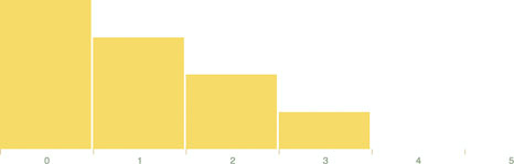
Let’s look at the data that histogram produces. One way to do this is by console.log(histoData) after you process it. You’ll see the array in figure 5.3. The array has been extended so that each array item has an x0 and x1 value that corresponds to the top and bottom thresholds of that bin. The array length indicates the number of items in that bin. And that’s all there is to that function, but it’s enough to provide us with sufficient drawing instructions to render the chart in figure 5.2.