concept function value in category deep learning

This is an excerpt from Manning's book Math and Architectures of Deep Learning.
How do we “adjust”
, b so that the value of loss L = E2 goes down? This is where gradients come in. For any function L (
Figure 3.9: The domain of
shown as a heat-map of function values. Gradients point radially outward as shown by the arrowed line. The deepness of the red color changes fastest along the gradient (i.e., radii). This is the direction to follow to rapidly reach lower values of the function represented by the heatmap.
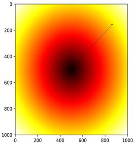
At any point on the domain, what is the direction along which the biggest change in function value occurs? The answer is along the direction of the gradient. The magnitude of the change corresponds to the magnitude of the gradient. In the current example, say we are at a point (w0,w1). There exists a level contour through this point - the circle with origin at center passing through (w0,w1). If we move along the circumference of this circle, i.e., along the tangent to this circle, the function value does not change at all. In other words, at any point, the tangent to the level contour through that point is the direction of minimal change. On the other hand, if we move perpendicular to the tangent, maximum change in the function value occurs. The perpendicular to the tangent is known as normal. This is the direction of the gradient. Gradient at any point on the domain is always normal to the level contour through that point, indicating the direction of maximum change in function value. In Figure 3.9, the gradients are all parallel to the radii of the concentric circles. T Recall that during training a machine learning model, we essentially define a loss function in terms of a tunable set of parameters and try to minimize the loss by adjusting (tuning) the parameters. We start at a random point and iteratively progress towards the minimum.
Geometrically, this can be viewed as starting at an arbitrary point on the domain and continuing to move in a direction that minimizes the function value. Of course, we would like to progress to the minimum of the function value in as few iterations as possible. In Figure 3.9 the minimum i at the origin, which is also the center of all the concentric circles. Wherever we start, we will have to alway travel radially inwards to reach the minimum (0, 0) of the function
.
In higher dimensions, level contours become level surfaces. Given any function