concept distance in category gnuplot

This is an excerpt from Manning's book Gnuplot in Action.
Figure 3.3. The average speed of the current world record holder, as a function of the distance. The speed has been calculated from the distance and the finishing time as part of the plot command, using an inline transformation: plot "records" u 2:($1/$2) w lp. (See listing 3.1 for the data.)

I’ll talk about data files and their permissible formats in more detail in chapter 4. For now, suffice to say that gnuplot expects data files to be whitespace-separated, column-oriented text files, with one line per record. Listing 3.1 shows an example: the world records (as of late 2014) for both men and women running events at a variety of distances. (Distances are in meters, and times are in seconds—the last two entries with the “odd” distances are for half-marathon and full-marathon races.)
Listing 3.1. Data for figure 3.1 (file: records)
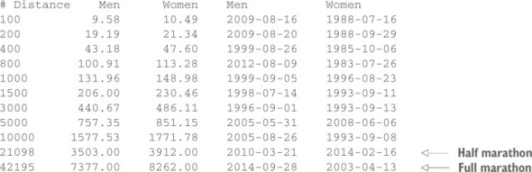
Figure 3.1 displays a plot of the finishing times for events up to 10,000 meters as a function of the distance, together with two function plots for comparison (the using, title, and w p directives were introduced in section 2.1.2):
For these reasons, you occasionally see the data represented in a stacked plot, as in figure 14.9, upper right. Here, the numbers for all products have been stacked on top of one another, so that the curve for (say) product 2 represents the total manufactured output for products 1 and 2 combined. By construction, lines in such plots never cross, and hence the graphs always have a neat appearance—which makes them popular in general-interest publications. Nevertheless, they have significant problems. Only two curves are easy to interpret: the bottom one (product 1) and the top one (total production). It’s exceptionally hard in such a stacked graph to estimate how the contributions from the individual components change over time. For example, how much of the sudden increase in total production after week 130 is due to product 4? It’s basically impossible to tell from this graph—you have to go back to the previous panel. Similarly, from this graph, it isn’t easy to see that the double-hump configuration starting in week 100 is due exclusively to product 2. (Judging the distance between closely spaced curves that vary a lot over the plot range is exceptionally difficult—see section 14.3.2.)

This is an excerpt from Manning's book Gnuplot in Action: Understanding Data with Graphs.
When using one of the five smoothing kernels from table 8.3, up to two additional parameters can be specified: dx and dy. These are used to rescale the coordinate differences when calculating the distance di = ( ((x-xi)/dx)2 + ((y-yi)/dy)2)1/2, where x and y are the coordinates of the current grid point and xi and yi are the coordinates of the i th data point. The value of dy defaults to the value of dx, which defaults to 1. The parameters dx and dy make it possible to control the radius over which data points contribute to a grid point in the units of the data itself.
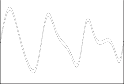
Figure 14.14 demonstrates the same point. Looking at the plot, the conclusion seems inevitable that the distance between the two curves varies, being largest close to the maxima and minima of the two curves, and in general increasing from left to right. Yet, in reality, the vertical distance between the two curves is exactly constant over the entire plot range: the graph shows the same function twice, shifted vertically by a constant amount.