concept hide layer in category Keras
This is an excerpt from Manning's book Probabilistic Deep Learning: With Python, Keras and TensorFlow Probability.
To get a first idea about an artificial NN, you can better imagine a neuron as a container for a number. The neurons in the input layer are correspondingly holding the numbers of the input data. Such input data could for example be the age (in years), income (in dollars), and height (in inches) of a customer. All neurons in the following layers get the weighted sum of the values from the connected neurons in the previous layer as their input. In general, the different connections aren’t equally important but have weights, which determine the influence of the incoming neuron’s value on the neuron’s value in the next layer. (Here we omit that this input is further transformed within the neuron). DL models are NNs, but they also have a large number of hidden layers (not just three as in the example from figure 1.2).
In this section, you will use the Maximum Likelihood principle to derive the loss function for regression problems. You will start off by revisiting the blood pressure example from chapter 3, where the input was the age of an american healthy woman and the output was a prediction of her systolic blood pressure (sbp). In chapter 3 you have used a simple NN without hidden layers to model a linear relationship between input and output. As the loss function you have used the mean square error. This choice of the loss function was explained by some handwaving arguments, but no hard facts were given to prove that this loss function is a good choice. In this chapter you will see that the MSE as a loss function directly results from the maximum likelihood principle. Further, using the maximum likelihood principle, we can go beyond the mean squared error loss and model data with non constant noise, known under the scary name heteroscedasticity in the statistics community. Don’t be afraid; understanding the maximum likelihood principle makes modeling (not spelling) heteroscedasticity a piece of cake.
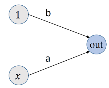
Figure 4.12 Simple linear regression as fully connected neural network without hidden layer computing the output directly from the input as out = a · x + b.
listing 4.6 A fully connected NN with hidden layers, two output nodes and a custom loss to fit the non-linear heteroscatic regression model from equation 4.6
import math
def my_loss(y_true,y_pred):  #A
  mu=tf.slice(y_pred,[0,0],[-1,1])              #B
  sigma=tf.math.exp(tf.slice(y_pred,[0,1],[-1,1]))   #C

  a=1/(tf.sqrt(2.*math.pi)*sigma)
  b1=tf.square(mu-y_true)
  b2=2*tf.square(sigma)
  b=b1/b2
  loss = tf.reduce_sum(-tf.math.log(a)+b,axis=0)
  return loss

model =  Sequential() #D
model.add(Dense(20, activation='relu',batch_input_shape=(None, 1)))
model.add(Dense(50, activation='relu'))
model.add(Dense(20, activation='relu'))
model.add(Dense(2, activation='linear'))
model.compile(loss=my_loss,optimizer="adam",metrics=[my_loss])#E