concept column in category machine learning

This is an excerpt from Manning's book Machine Learning Bookcamp.
We can use this attribute only for columns with string values inside. This is exactly why we first select such columns in B.
In Pandas, a DataFrame is simply a table: a data structure with rows and columns (figure D.1).
Figure D.3 Two ways of accessing a column of a DataFrame: (A) the “dot” notation and (B) the “brackets” notation.
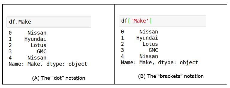
The bracket notation is also more flexible: we can keep the name of a column in a variable and use it to access its content:
col_name = 'Engine HP'
df[col_name]
If we need to select a subset of columns, we again use brackets, but with a list of names instead of a single string:

This is an excerpt from Manning's book Machine Learning with R, the tidyverse, and mlr.
What we mean by rows, columns, cases, and variables
Listing 2.3. Selecting columns using select()
library(dplyr)

selectedData <- select(CO2tib, 1, 2, 3, 5)

selectedData

# A tibble: 84 x 4
   Plant Type   Treatment  uptake
 * <ord> <fct>  <fct>       <dbl>
 1 Qn1   Quebec nonchilled   16
 2 Qn1   Quebec nonchilled   30.4
 3 Qn1   Quebec nonchilled   34.8
 4 Qn1   Quebec nonchilled   37.2
 5 Qn1   Quebec nonchilled   35.3
 6 Qn1   Quebec nonchilled   39.2
 7 Qn1   Quebec nonchilled   39.7
 8 Qn2   Quebec nonchilled   13.6
 9 Qn2   Quebec nonchilled   27.3
10 Qn2   Quebec nonchilled   37.1
# ... with 74 more rows

This is an excerpt from Manning's book Machine Learning for Business: Using Amazon SageMaker and Jupyter.
You’ll find the most correlated columns by applying another pandas function called corr. You apply the corr function by appending .corr() to the pandas DataFrame you named encoded_data in listing 2.5. After the function, you need to provide the name of the column you are attempting to predict. In this case, the column you are attempting to predict is the tech_approval_required column. Listing 2.6 shows the code that does this. Note that the .abs() function at the end of the listing is simply turning all of the correlations positive.
Listing 2.6. Identifying correlated columns
corrs = encoded_data.corr()[
            'tech_approval_required'
        ].abs()                        #1
columns = corrs[corrs > .1].index      #2
corrs = corrs.filter(columns)          #3
corrs                                  #4
The code in listing 2.6 identifies the columns that have a correlation greater than 10%. You don’t need to know exactly how this code works. You are simply finding all of the columns that have a correlation greater than 10% with the tech_approval_required column. Why 10%? It removes the irrelevant noise from the dataset which, while this step does not help the machine learning algorithm, improves your ability to talk about the data in a meaningful way. With fewer columns to consider, you can more easily prepare an explanation of what the algorithm is doing.
Table 2.5 shows the columns with a correlation greater than 10%.
Table 2.5. Correlation with predicted value (view table figure)
Column name
Correlation with predicted value
tech_approval_required 1.000000 role_non-tech 0.122454 role_tech 0.122454 product_Chair 0.134168 product_Cleaning 0.191539 product_Desk 0.292137 product_Desktop Computer 0.752144 product_Keyboard 0.242224 product_Laptop Computer 0.516693 product_Mouse 0.190708 Now that you have identified the most highly correlated columns, you need to filter the encoded_data table to contain just those columns. You do so with the code in listing 2.7. The first line filters the columns to just the correlated columns, and the second line displays the table when you run the code. (Remember, to run the code, insert your cursor in the cell and press
.)

You can see from this time series that the date is on the left and my weight is on the right. If you wanted to record the time series of body weight for your entire family, for example, you would add a column for each of your family members. In table 6.2, you can see my weight and the weight of each of my family members over the course of a year.