concept frequency in category python

This is an excerpt from Manning's book Math for Programmers: 3D graphics, machine learning, and simulations with Python.
We also use a single channel, meaning we only play one sound wave as opposed to stereo audio, which produces two sound waves simultaneously, one in the left speaker and one in the right. The other thing we configure is the bit depth of the sound. While frequency is analogous to the resolution of an image, bit depth is like the number of allowable pixel colors, more bit depth means a more refined range of sound intensities. We used three numbers between 0 and 256 for the color of a pixel, but here, we use a single 16-bit number to represent the sound intensity at a moment in time. With these parameters selected, the first step in our code is to import PyGame and initialize the sound library:
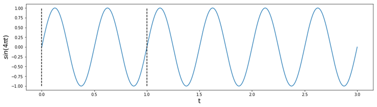
Figure 13.13: The graph of sin(4𝜋t) is sinusoidal, repeating itself twice in every unit of t for a frequency of 2.
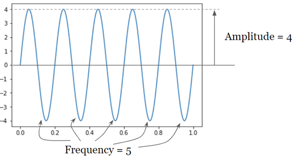
We can test this, for example, by making a sinusoidal function with a frequency of 5 and an amplitude of 4, and plotting it (figure 13.14) from t = 0 to t = 1:
>>> plot_function(make_sinusoid(5,4),0,1)Figure 13.14: The graph of make_sinusoid(5,4) has a height (amplitude) of 4 and repeats itself 5 times from t = 0 to t = 5, so it has a frequency of 5.
Next, we work with the sound wave function that is the result of make_sinusoid(441,8000) having a frequency of 441 Hz and an amplitude of 8,000.
This is an excerpt from Manning's book Mastering Large Datasets with Python: Parallelize and Distribute Your Python Code.
We can use frequencies from the toolz library to get counts of the unique elements of a sequence.
frequencies
Figure 6.7 shows that, like filter, the frequencies process will use different functions for the accumulation and combination steps. For the accumulation step, we’ll use the make_counts function from listing 5.7. For the combination step, we’ll have to write an entirely new function. This function will have to go through the unique keys of our two dicts and add the values of those keys together in a new dict. We can see that even though our frequencies process can take iterables with any number of types of elements, we’ll always be passing dicts to our combination function because that’s the type that our make_counts accumulation function returns.
We can see the same limited changes between linear and parallel frequencies, as shown in the following listing. Again, what’s important is that we pass the combination function and the parallel map.
Listing 6.11. Implementing frequencies in parallel with parallel reduce
import dill as pickle                                           #1
from pathos.multiprocessing import ProcessingPool as Pool
from toolz.sandbox.parallel import fold
from random import choice                                       #2
from functools import reduce


def combine_counts(left, right):                                #3
  unique_keys = set(left.keys()).union(set(right.keys()))
  return {k:left.get(k, 0)+right.get(k, 0) for k in unique_keys}

def make_counts(acc, nxt):                                      #4
    acc[nxt] = acc.get(nxt,0) + 1
    return acc

xs = (choice([1, 2, 3, 4, 5, 6]) for _ in range(500000))        #5

with Pool() as P:                                               #6
    fold(make_counts, xs, {},
         map=P.imap, combine=combine_counts)
rand_nums = (choice([1, 2, 3, 4, 5, 6]) for _ in range(500))
reduce(make_counts, rand_nums, {})                              #7
# {6: 87, 1: 59, 5: 88, 4: 85, 3: 93, 2: 88}
We can see again how similar the parallel reduce and the linear reduce are. With the key exception of the combination function and the parallel map, they both use the same parameters: the same accumulation function, the same data inputs, and the same initializer. Across all three examples—parallel reduce summation, parallel reduce filter, and parallel reduce frequencies—we have seen our combination functions increase in complexity. Getting this combination function right is the key to successfully using parallel reduce.