concept prediction in category R

This is an excerpt from Manning's book Machine Learning with R, the tidyverse, and mlr.
Columns that contain measurements made on each case are referred to as variables. When we’re trying to predict the value of one variable based on its relationships with the others, we use terms to distinguish between the variable we want to predict and the ones we are using to make the predictions. Statisticians call the variable we’re trying to predict the dependent variable, while the variables we used to make these predictions are called the independent variables. In data science, you might be more likely to hear the term outcome or response variable for the dependent variable and predictor variables or features for the independent variables. I use the data science terminology throughout the book.
Listing 4.14. Using our model to make predictions on new data
data(titanic_test, package = "titanic")

titanicNew <- as_tibble(titanic_test)

titanicNewClean <- titanicNew %>%
  mutate_at(.vars = c("Sex", "Pclass"), .funs = factor) %>%
  mutate(FamSize = SibSp + Parch) %>%
  select(Pclass, Sex, Age, Fare, FamSize)

predict(logRegModel, newdata = titanicNewClean)

Prediction: 418 observations
predict.type: prob
threshold: 0=0.50,1=0.50
time: 0.00
     prob.0     prob.1 response
1 0.9178036 0.08219636        0
2 0.5909570 0.40904305        0
3 0.9123303 0.08766974        0
4 0.8927383 0.10726167        0
5 0.4069407 0.59305933        1
6 0.8337609 0.16623907        0
… (#rows: 418, #cols: 3)
By the end of this chapter, you’ll understand the difference between ordinary decision trees and ensemble methods, such as random forest and gradient boosting, which combine multiple trees to make predictions. Finally, as this is the last chapter in the classification part of the book, you’ll learn what benchmarking is and how to use it to find the best-performing algorithm for a particular problem. Benchmarking is the process of letting a bunch of different learning algorithms fight it out to select the one that performs best for a particular problem.
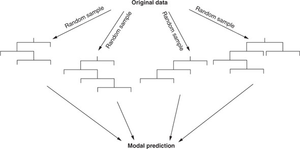
So why does training sub-models on bootstrap samples of the training set help us? Imagine that cases are distributed over their feature space. Each time we take a bootstrap sample, because we are sampling with replacement, we are more likely to select a case near the center of that distribution than a case that lies near the extremes of the distribution. Some of the bootstrap samples may contain many extreme values and make poor predictions on their own, but here’s the second crucial part of bagging: we aggregate the predictions of all these models. This simply means we let them all make their predictions and then take the majority vote. The effect of this is a sort of averaging out of all the models, which reduces the impact of noisy data and reduces overfitting. Bagging for decision trees is illustrated in figure 8.1.
In this section, I’ll explain the principle of the stacking ensemble technique and how it is used to combine predictions from multiple algorithms. Stacking is an ensemble technique that, while valuable, isn’t as commonly used as bagging and boosting. For this reason, I won’t discuss it in a lot of detail, but if you’re interested in learning more, I recommend Ensemble Methods: Foundations and Algorithms by Zhi-Hua Zhou (Chapman and Hall/CRC, 2012).

This is an excerpt from Manning's book Practical Data Science with R, Second Edition.
4Normally, we’d evaluate the model against a test set (data that wasn’t used to build the model). In this example, for simplicity, we'll evaluate the model against the training data (data that was used to build the model). Also note we are following a convention that we will use when plotting: predictions are the x-axis, which for tables means predictions are the column names. Be aware that there are other conventions for confusion matrices.
Before publicly sharing predictions, you want to inspect both the predictions and model for quality. We recommend plotting the actual y (in this case, predicted income) that you’re trying to predict as if it were a function of your prediction. In this case, plot log10(PINCP) as if it were a function of predLogPINCP. If the predictions are very good, then the plot will be dots arranged near the line y=x, which we call the line of perfect prediction (the phrase is not standard terminology; we use it to make talking about the graph easier). The steps to produce this, illustrated in figure 7.6, are shown in the next listing.
Listing 7.3. Plotting residuals income as a function of predicted log income
ggplot(data = dtest, aes(x = predLogPINCP,
                     y = predLogPINCP - log10(PINCP))) +
  geom_point(alpha = 0.2, color = "darkgray") +
  geom_smooth(color = "darkblue") +
  ylab("residual error (prediction - actual)")
Why are the predictions, not the true values, on the x-axis?
A graph that plots predictions on the x-axis and either true values (as in figure 7.6) or residuals (as in figure 7.7) on the y-axis answers different questions than a graph that puts true values on the x-axis and predictions (or residuals) on the y-axis. Statisticians tend to prefer the graph as shown in figure 7.7. A residual graph with predictions on the x-axis gives you a sense of when the model may be under- or overpredicting, based on the model’s output.

This is an excerpt from Manning's book Deep Learning with R.
To control something, first you need to be able to observe it. To control the output of a neural network, you need to be able to measure how far this output is from what you expected. This is the job of the loss function of the network, also called the objective function. The loss function takes the predictions of the network and the true target (what you wanted the network to output) and computes a distance score, capturing how well the network has done on this specific example (see figure 1.8).
You can visualize their interaction as illustrated in figure 3.1: the network, composed of layers that are chained together, maps the input data to predictions. The loss function then compares these predictions to the targets, producing a loss value: a measure of how well the network’s predictions match what was expected. The optimizer uses this loss value to update the network’s weights.
Each entry in predictions is a vector of length 46: