concept state in category reinforcement learning

This is an excerpt from Manning's book Grokking Deep Reinforcement Learning.
variables that make up the environment. This set of variables and all the possible values that they can take are referred to as the state space. A state is an instantiation of the state space, a set of values the variables take.
Interestingly, often, agents don’t have access to the actual full state of the environment. The part of a state that the agent can observe is called an observation. Observations depend
on states but are what the agent can see. For instance, in the manipulator example, the agent may only have access to camera images. So, while there is an exact location of each object, the agent doesn’t have access to this specific state. Instead, the observations the agent perceives are derived from the states. You’ll often see in the literature observations and states being used interchangeably, including in this book. I apologize in advance for the inconsistencies. Simply know the differences and be aware of the lingo, that’s what matters.
Figure 1.6 States vs. observations

At each state, the environment makes available a set of actions the agent can choose from. The agent influences the environment through these actions. The environment may change states as a response to the agent’s action. The function that is responsible for this mapping is called the transition function. The environment may also provide a reward signal as a response. The function responsible for this mapping is called the reward function. The set of transition and reward functions is referred to as the model of the environment.
If we don’t use discounting, well, the return would just be 1 for this trajectory and all trajectories that end in the right-most cell, state 6, and 0 for all trajectories that terminate in the left-most cell, state 0.
Something that’d help us compare policies is to put numbers to states for a given policy. That is, if we are given a policy and the MDP, we should be able to calculate the expected return starting from every single state (we care mostly about the START state). So, how can we calculate how valuable being in a state is? For instance, if our agent is in state 14 (to the left of the GOAL,) how is that better than being in state 13 (to the left of 14)? And precisely how much better is it? More importantly, under which policy we’d have better results, the “Go get it” or the “Careful” policy?
Let’s give it a quick try with the “Go get it” policy. What is the value of being in state 14 under the “Go get it” policy?
Figure 3.11 What’s the value of being in state 14 when running the “Go get it” policy?
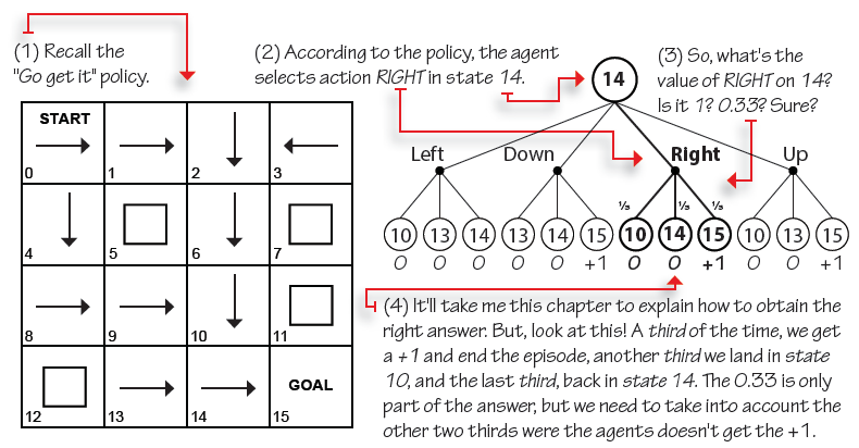
Okay, so it is not that straightforward to calculate the value of state 14 when following the “Go get it” policy because of the dependence on the values of other states (10 and 14 in this case), which we don’t have either. It’s like the chicken or the egg problem. Let’s keep going.
We defined the return as the sum of rewards the agent obtains from a trajectory. Now, this return can be calculated without paying attention to the policy the agent is following, you just sum all of the rewards obtained, and you are good to go. But, the number we are looking for now is the expectation of returns (from state 14) if we follow a given policy π. Remember, we are under stochastic environments, so we must account for all the possible ways the environment can react to our policy! That’s what an expectation gives us.
We now define the value of a state s whn following a policy π: the value of a state s under policy π is the expectation of returns if the agent follows policy π starting from state s.
This is an excerpt from Manning's book Deep Reinforcement Learning in Action.
The state is a snapshot of the environment that the agent has access to and uses to make decisions. The environment is often a set of constantly changing conditions, but we can sample from the environment, and these samples at particular times are the state information of the environment we give to the agent.
Figure 2.6. A computational graph for a simple 10-armed contextual bandit. The get_state() function returns a state value, which is transformed into a one-hot vector that becomes the input data for a two-layer neural network. The output of the neural network is the predicted reward for each possible action, which is a dense vector that is run through a softmax to sample an action from the resulting probability distribution over the actions. The chosen action will return a reward and updates the state of the environment. θ1 and θ2 represent the weight parameters for each layer. The
,
, and
symbols denote the natural numbers (0, 1, 2, 3, ...), the real numbers (a floating-point number, for our purposes), and a probability, respectively. The superscript indicates the length of the vector, so

Initially our neural network will produce a random vector such as [1.4, 50, 4.3, 0.31, 0.43, 11, 121, 90, 8.9, 1.1] when in state 0. We will run softmax over this vector and sample an action, most likely action 6 (from actions 0 through 9), since that is the biggest number in the example vector. Choosing action 6 will generate a reward of say 8. Then we train our neural network to produce the vector [1.4, 50, 4.3, 0.31, 0.43, 11, 8, 90, 8.9, 1.1], since that is the true reward we received for action 6, leaving the rest of the values unchanged. The next time when the neural network sees state 0, it will produce a reward prediction for action 6 closer to 8. As we continually do this over many states and actions, the neural network will eventually learn to predict accurate rewards for each action given a state. Thus, our algorithm will be able to choose the best action each time, maximizing our rewards.
We’ll run the softmax function over the model’s output to generate a probability distribution over the actions. We’ll then select an action using the environment’s choose_arm(...) function, which will return the reward generated for taking that action; it will also update the environment’s current state. We’ll turn the reward (which is a non-negative integer) into a one-hot vector that we can use as our training data. We’ll then run one step of backpropagation with this reward vector, given the state we gave the model. Since we’re using a neural network model as our action-value function, we no longer have any sort of action-value array storing “memories;” everything is being encoded in the neural network’s weight parameters. The whole train function is shown in the following listing.
Listing 2.10. The main training loop
def train(env, epochs=5000, learning_rate=1e-2):
    cur_state = torch.Tensor(one_hot(arms,env.get_state()))             #1
    optimizer = torch.optim.Adam(model.parameters(), lr=learning_rate)
    rewards = []
    for i in range(epochs):
        y_pred = model(cur_state)                                       #2
        av_softmax = softmax(y_pred.data.numpy(), tau=2.0)              #3
        av_softmax /= av_softmax.sum()                                  #4
        choice = np.random.choice(arms, p=av_softmax)                   #5
        cur_reward = env.choose_arm(choice)                             #6
        one_hot_reward = y_pred.data.numpy().copy()                     #7
        one_hot_reward[choice] = cur_reward                             #8
        reward = torch.Tensor(one_hot_reward)
        rewards.append(cur_reward)
        loss = loss_fn(y_pred, reward)
        optimizer.zero_grad()
        loss.backward()
        optimizer.step()
        cur_state = torch.Tensor(one_hot(arms,env.get_state()))         #9
    return np.array(rewards)
Go ahead and run this function. When we train this network for 5,000 epochs, we can plot the moving average of rewards earned over the training time (see figure 2.7; we omitted the code to produce such a graph). Our neural network indeed learns a fairly good understanding of the relationship between states, actions and rewards for this contextual bandit. The maximum reward payout for any play is 10, and our average is topping off around 8.5, which is close to the mathematical optimum for this particular bandit. Our first deep reinforcement learning algorithm works! Okay, it’s not a very deep network, but still!
Value functions are functions that map a state or a state-action pair to the expected value (the expected reward) of being in some state or taking some action in some state. You may recall from statistics that the expected reward is just the long-term average of rewards received after being in some state or taking some action. When we speak of the value function, we usually mean a state-value function.
Table 2.7. The state-value function (view table figure)
Math
English
Vπ: s → E(R|s,π), A value function, Vπ, is a function that maps a state, s, to the expected rewards, given that we start in state s and follow some policy, π. This is a function that accepts a state, s, and returns the expected reward of starting in that state and taking actions according to our policy, π. It may not be immediately obvious why the value function depends on the policy. Consider that in our contextual bandit problem, if our policy was to choose entirely random actions (i.e., sample actions from a uniform distribution), the value (expected reward) of a state would probably be pretty low, since we’re definitely not choosing the best possible actions. Instead, we want to use a policy that is not a uniform distribution over the actions, but is the probability distribution that would produce the maximum rewards when sampled. That is, the policy is what determines observed rewards, and the value function is a reflection of observed rewards.
