Variational inference

As explained in Machine Learning Algorithms in Depth

Accurate variational inference uses richer variational models than fully factorized approximations to improve posterior approximation quality.

Variational inference (VI) approximates a difficult posterior with a distribution that is easier to compute. Choose a tractable family q(z), give it trainable parameters, and optimize those parameters so q(z) approaches the posterior p(z|x). Unlike Markov chain Monte Carlo (MCMC), which approximates a posterior using samples, VI turns inference into an optimization problem. section 3.0 section 1.6

The choice of q limits the approximation. A mean-field q is fully factorized, which speeds computation but restricts the posterior shapes it can represent. For greater accuracy, the aim is to improve the variational approximation rather than rely only on that factorization; no particular richer family or update rule is specified here. section 3.0 section 3.1

KL divergence measures a mismatch between distributions, but its direction matters. On a multimodal posterior, forward KL can favor a broad q that covers low-density space between modes; reverse KL can favor q concentrated on one mode. Accuracy therefore depends both on the variational family and on what the objective rewards. section 1.4.1 section 3.1

Let x denote observations and z latent variables. Jensen’s inequality gives an evidence lower bound (ELBO) to maximize when learning q. One interpretation balances high joint probability against the entropy of q; another expresses a likelihood term alongside divergence from the prior. The bound tightens as q better approximates the posterior, and expectations under q can be estimated by drawing samples from q. section 3.1

Topic inference with variational Bayes

For latent Dirichlet allocation, coordinate-ascent updates optimize variational parameters. An online version updates document-level parameters, then blends a proposed global update with its previous value. A from-scratch implementation tracks increasing ELBO across mean-field iterations and displays inferred topics as word clouds. This demonstrates the factorized baseline, not an implemented richer variational family. section 9.1.1

Figure 3.2 Forward KL (left) q(x) overestimates the support, while reverse KL (right) q(x) locks onto a mode.

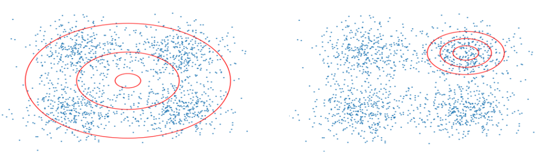
Compare the broad forward-KL fit with the reverse-KL fit concentrated on a mode; the figure makes the objective’s effect on approximation quality visible. section 3.1

How Machine Learning Algorithms in Depth covers it

How deep it goes

Derives an ELBO and implements mean-field variational Bayes for LDA, but does not specify a richer-family update rule.

Examples

Uses Gaussian-mixture KL fits and a from-scratch LDA implementation with ELBO plots and topic word clouds.

What it assumes

Assumes familiarity with posterior distributions and probability while introducing tractable approximations and deriving the objective with Jensen’s inequality.

What you can do after

Build it from scratch for mean-field LDA and evaluate approximation behavior through the ELBO and KL direction.

How it connects

Connects KL divergence, the evidence lower bound, mean-field approximation, Bayesian posterior inference, and latent Dirichlet allocation.

liveBookmanning.com

Read Machine Learning Algorithms in Depth on liveBook Get the book at manning.com

Also explained in

• 

  liveBookmanning.com
  Causal AIVariational inference approximates a target probability distribution by optimizing the parameters of a tractable distribution or stochastic process.

Compare how 2 books explain variational inference →

Related concepts

• stochastic variational inferenceincludes · Stochastic variational inference is a variational inference technique that optimizes an objective using stochastic estimates, often computed from randomly sampled data subsets.
• Kullback–Leibler divergenceuses · Kullback–Leibler divergence is a nonnegative, directed measure of the information lost when one probability distribution approximates another, computed as an expected log ratio under the first distribution.
• evidence lower bounduses · The evidence lower bound is a variational objective that lower-bounds a model’s log marginal likelihood and is optimized to approximate the posterior distribution.
• markov chain monte carloalternative to · Markov chain Monte Carlo is a family of sampling algorithms that generate samples using a Markov chain whose stationary or limiting distribution is a target probability distribution.
• approximate distributionuses · An approximate posterior distribution is a tractable probability distribution selected or optimized to represent an intractable posterior distribution over unknown quantities.
• optimizationuses · Optimization is the systematic selection or adjustment of values, actions, or system designs to improve a specified objective, often subject to constraints.

This explainer was generated by Manning's knowledge graph from the text of Machine Learning Algorithms in Depth. The section links point to the parts of the book it draws on.