Affine transform

As explained in Geometry for Programmers

An affine transformation is a geometric mapping that preserves straight lines and parallelism while allowing translation, rotation, scaling, and shearing.

An affine transform moves a 2D point with two linear expressions plus constant offsets: xt = a11xi + a12yi + a13 and yt = a21xi + a22yi + a23. The extra constants let the transform shift shapes instead of keeping everything anchored at the origin. Think of it as a linear transform you can carry around the plane. section 4.2.2

Parallel lines stay parallel. Rotation and scaling fit the same formula, and translation is the simple case where the linear part is the identity and only the offsets change. This makes affine transforms a practical middle ground: more flexible than a purely linear transform while retaining straightforward arithmetic. section 4.2.2 section 4.2.5

Figure 4.13 Three examples of affine transformations, which look a lot like linear ones but now have translations

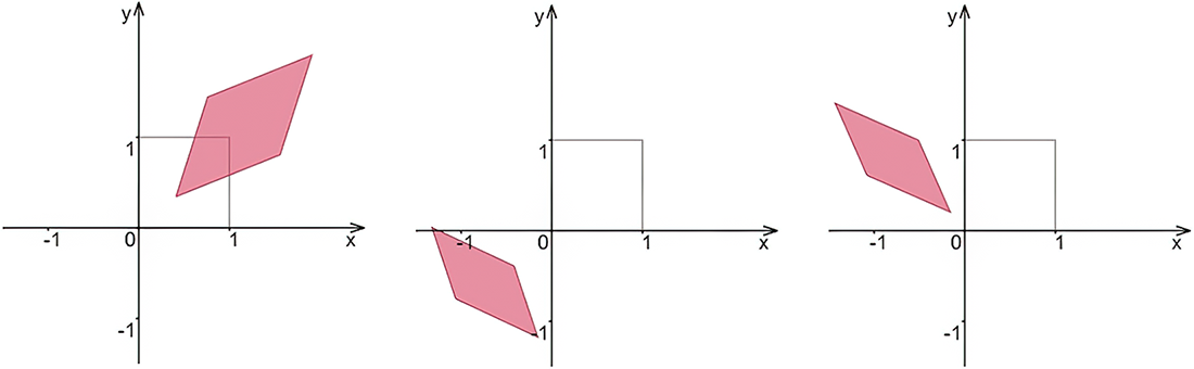
Compare the transformed shapes: they resemble linear-transform results, but translation lets their position change freely. section 4.2.2

A 2D affine transform has six coefficients. Matching three source points to three destination points supplies six coordinate equations—one x and one y equation per point—so the coefficients can be solved symbolically. The resulting formulas share a divisor, but the important engineering idea is simple: three point correspondences determine the transform used here. section 4.2.2

Normalize a triangle before testing a point

Map an arbitrary triangle’s three vertices to (0, 0), (1, 0), and (0, 1). Precompute the six affine coefficients once per triangle, then transform each candidate point with four multiplications and six additions. The transformed point is inside when xt > 0, yt > 0, and xt + yt < 1. This avoids using a full projective transform when three points are enough. section 4.4.2

Figure 4.22 A triangle in space versus the same triangle in its own basis

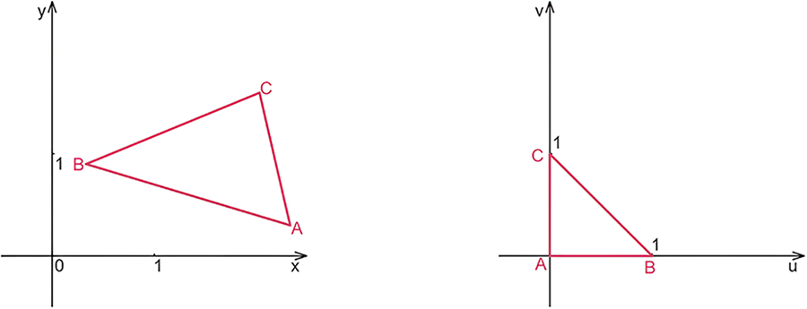
The figure shows why mapping a triangle into its own standard basis makes the final containment check small and regular. section 4.4.2

Homogeneous coordinates provide a convenient matrix representation. Translation, rotation, and scaling can then use one matrix-multiplication path rather than separate functions. In 3D, the same arrangement uses four-number homogeneous points and 4 × 4 matrices. Matrix composition can also combine several transformations into one. section 4.3.2

How Geometry for Programmers covers it

How deep it goes

Derives six coefficients from three 2D point pairs and implements point mapping, then extends representation to homogeneous matrices.

Examples

Uses three moved 2D points, affine-transformation figures, and an arbitrary triangle mapped to a standard basis.

What it assumes

Builds from linear transformations and coordinate equations, while introducing translation through added constant terms.

What you can do after

Apply it via SymPy or matrix multiplication to fit 2D transforms and preprocess triangles for containment checks.

How it connects

Connects linear transformations, translation, rotation, scaling, homogeneous coordinates, matrix multiplication, and projective transformations.

liveBookmanning.com

Read Geometry for Programmers on liveBook Get the book at manning.com

Related concepts

• linear layerimplemented by · A linear layer is a neural-network layer that maps input features to outputs by a learned affine transformation, typically connecting each output to every input feature.
• quantizationused by · Quantization maps numerical values to a finite set of discrete representations, often using reduced precision to lower model storage or computation requirements.
• linear regressionused by · Linear regression is a statistical modeling method that estimates a continuous response as a linear combination of predictor variables and fitted coefficients.
• geometric transformationkind of · A geometric transformation is a mapping or operation that changes or expresses the position, orientation, scale, shape, or coordinate representation of geometric objects.
• translationuses · A translation is a geometric transformation that moves every point by the same displacement without changing an object’s shape or orientation.

This explainer was generated by Manning's knowledge graph from the text of Geometry for Programmers. The section links point to the parts of the book it draws on.