AlexNet

As explained in Sutskever's List

AlexNet is a convolutional neural network architecture that achieved a landmark result in large-scale image classification.

In 2012, AlexNet changed what counted as a promising approach to image recognition. Alex Krizhevsky, Ilya Sutskever, and Geoffrey Hinton trained a convolutional neural network on ImageNet images rather than relying on handcrafted visual features. Its 15.3% top-5 error in the ImageNet challenge was far below the runner-up’s 26.2%. Top-5 error means the correct label was absent from the model’s five highest-ranked guesses. section 2.0 section 2.5

The architecture had about 60 million trainable parameters and five initial convolutional layers. Those layers learned features from images, replacing the need to specify features by hand. Convolution and pooling progressively reduced spatial resolution; fully connected layers then fed a 1,000-category output. The original design split work across two GPUs, an engineering constraint visible in its two-stream diagram. section 2.5.1

Figure 2.3 The AlexNet architecture (cropped in the original paper). The numbers indicate spatial dimensions and channel depth at each stage. The input image (224 × 224 × 3 RGB) passes through a series of convolutional and pooling layers that progressively reduce spatial resolution (224→55→27→13) while increasing channel depth. Early downsampling is driven by the first convolutional layer (11 × 11 filters with a stride of 4), followed by max pooling layers (3 × 3 windows with a stride of 2) that further reduce spatial dimensions. The stride determines how far a filter moves across the input at each step, controlling how densely the image is sampled and how quickly spatial resolution is reduced. Filter sizes (11, 5, 3) are depicted as cubes and define the local receptive field of each convolution. The two horizontal streams reflect the model’s original two-GPU training setup, where feature maps were split across devices (e.g., 48 + 48 = 96 channels). The fully connected layers (4096 neurons, implemented as 2048 + 2048 across GPUs) feed into a 1000-way output for ImageNet classification. Used with permission granted by the lead author (Alex Krizhevsky).

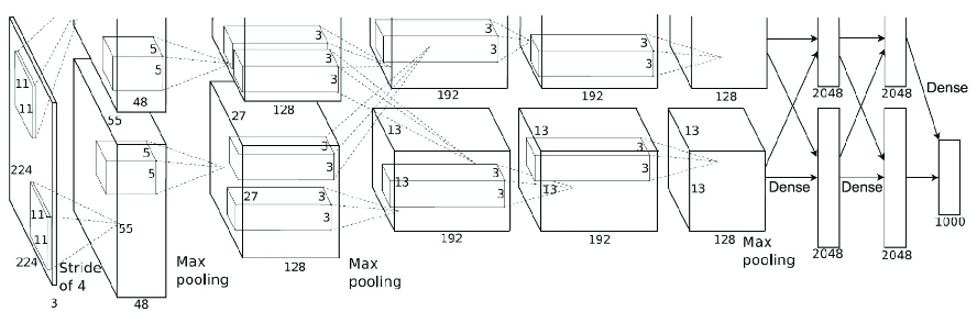
Follow the image from its 224 × 224 × 3 input through shrinking spatial dimensions to the 1,000-way output. The paired streams show how feature maps were divided between GPUs. section 2.5.1

Training a network this large required practical choices, not just more layers:

• Rectified linear units (ReLUs) set negative inputs to zero but leave positive inputs unchanged. Compared with tanh activations, they reduced saturation and made convergence six times faster in a controlled experiment. section 2.5.2
• Dropout randomly disabled half the neurons in the first two fully connected layers during each training iteration, countering overfitting where many of the model’s parameters were concentrated. section 2.5.2

The result challenged the idea that a larger image dataset alone would rescue existing methods: ImageNet performance had stalled despite its scale, while handcrafted-feature approaches had little room to improve. By the next year, nearly all ImageNet competition entries used CNNs. AlexNet’s lasting lesson was that architecture and trainability determined how much could be learned from abundant data; later CNNs pushed the benchmark further. section 2.5.5

How Sutskever's List covers it

How deep it goes

Explains architecture, training choices, and benchmark impact, including parameter scale and GPU splitting, without deriving the network mathematically.

Examples

Uses ImageNet top-5 error rates, an architecture diagram, and a tanh-versus-ReLU convergence experiment.

What it assumes

Defines parameters and neurons in plain language and contrasts activation functions rather than requiring a mathematical derivation.

What you can do after

Evaluate/understand it by relating AlexNet’s feature learning and training choices to its ImageNet result and subsequent CNN adoption.

How it connects

Connects convolutional neural networks to feature engineering, ReLU, dropout, overfitting, ImageNet, and later architectures such as ResNet.

liveBookmanning.com

Read Sutskever's List on liveBook Get the book at manning.com

Related concepts

• data augmentationuses · Data augmentation is the process of adding or deriving examples, variables, or associated information from existing data to increase its variety or support subsequent analysis or computation.
• ReLUuses · ReLU, or rectified linear unit, is an activation function that maps an input x to max(0, x).
• language modeluses · A language model is a computational model that represents patterns in linguistic tokens to estimate sequence probabilities and predict or generate language from context.
• dropoutuses · Dropout is a neural-network regularization technique that randomly suppresses units, connections, or activations during training to reduce overfitting.
• linear layerhas part · A linear layer is a neural-network layer that maps input features to outputs by a learned affine transformation, typically connecting each output to every input feature.
• vision modelkind of · A vision model is a machine-learning model that processes visual data, such as images or video, to analyze, generate, or extract information.

This explainer was generated by Manning's knowledge graph from the text of Sutskever's List. The section links point to the parts of the book it draws on.