Bayesian hypothesis testing treats hypotheses as competing models. It combines prior probabilities with the likelihood of observed data to produce posterior probabilities and compare how well each model explains what happened. section 11.11 section 11.6
A Bayesian hypothesis test typically proceeds by:
- Define both hypotheses explicitly, including the probability distribution each model assigns to possible outcomes. section 11.5
- Compute each hypothesis’s marginal likelihood, p(D | H), by averaging the likelihood over its possible parameter values. section 11.5
- Compare the marginal likelihoods with a Bayes factor, which quantifies relative evidence for either hypothesis rather than only rejecting one. section 11.11 section 11.5
- Combine the evidence with prior probabilities when the question concerns posterior belief or a decision. section 11.7 section 11.11
A conversion-rate comparison
One hypothesis fixes a conversion rate at 0.1; another assigns it a Beta(1, 1) distribution. A Bayes factor can favor the baseline model five to one, indicating substantial but inconclusive evidence rather than ruling out the alternative. More complex marginal likelihoods may require Monte Carlo or variational approximations. section 11.5
Avoiding the prosecutor’s paradox
A very small probability of seeing evidence if a defendant is innocent, p(D | H0), does not equal the probability of innocence given that evidence, p(H0 | D). Posterior odds also require alternative explanations and prior probabilities. section 11.7
Figure 11.3 Two competing hypotheses about the conversion rate 𝑟. The first hypothesis states that 𝑟 is equal to 0.1, while the second states that 𝑟 Follows a Beta(1, 1) distribution.
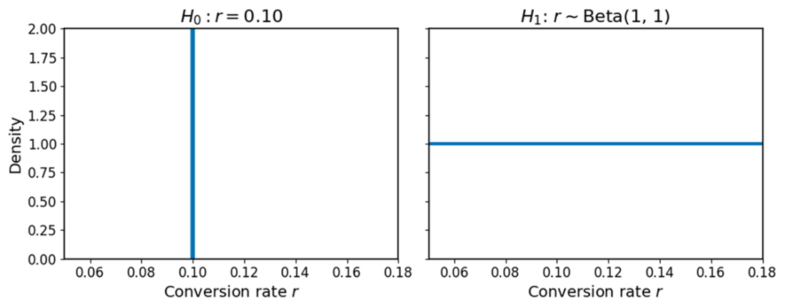
Compare the two conversion-rate hypotheses visually before interpreting their Bayes factor. section 11.5
