Beta (βₜ) is the per-step coefficient that controls how much noise enters a diffusion process. At each timestep, the previous data is scaled by √(1−βₜ), then random noise is added with scale √βₜ. As the schedule progresses, the original structure fades and the data becomes increasingly distorted. section 10.5
A beta schedule determines how diffusion behaves:
- Increase βₜ across timesteps to accumulate more total noise and reduce the influence of the original data. section 10.5
- Use a linear schedule by starting at a small β₀ and increasing to a larger βₜ value. section 10.5
- Treat the schedule as important: different beta values can affect the training outcome. section 10.5
- Combine schedule values into cumulative terms to compute the complete forward process in closed form. section 10.5 section 10.10
A 1,000-step linear schedule
A PyTorch schedule can span 1,000 steps, from β₀ = 0.0001 to β₉₉₉ = 0.02. Applying these values gradually transforms a structured set of points into noise; snapshots at steps 0, 250, 500, 800, and 999 make the progression visible. section 10.5
Figure 10.5 The forward diffusion process equation
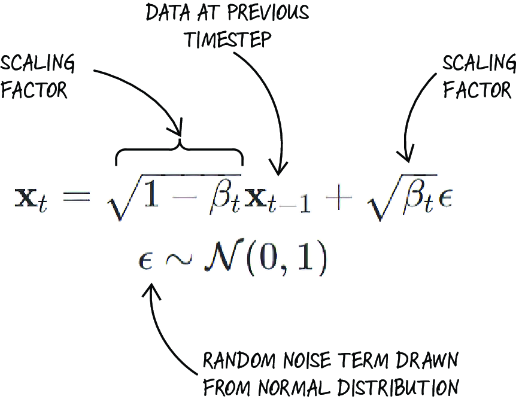
Use the forward diffusion equation to see exactly where βₜ scales retained data and newly added noise. section 10.5
# In[]:
def linear_beta_schedule(timesteps, start=0.0001, end=0.02):
    return torch.linspace(start, end, timesteps)
T = 1000
betas = linear_beta_schedule(T)
print(betas[0], betas[10], betas[T-1])

# Out[]:
tensor(1.0000e-04) tensor(0.0003) tensor(0.0200)
Inspect the compact PyTorch implementation of a linear beta schedule and its endpoint values. section 10.5
alphas = 1. - betas                                   #1
alphas_cumprod = torch.cumprod(alphas, dim=0)    #2
sqrt_alphas_cumprod = torch.sqrt(alphas_cumprod)
sqrt_one_minus_alphas_cumprod = torch.sqrt(1. - alphas_cumprod)

def reshape_for_x(a, x):     #3
    ones_to_broadcast = len(x.shape) - 1
    # python unpacking performed here
    return a.view(-1, *([1] * ones_to_broadcast)).to(x.device)

device = torch.device("cuda" if torch.cuda.is_available() else "cpu")
def forward_diffusion_sample(x, t):
    x = x.to(device)
    noise = torch.randn_like(x)
    sqrt_alphas_cumprod_t = reshape_for_x(sqrt_alphas_cumprod[t], x)
    sqrt_one_minus_alphas_cumprod_t =  reshape_for_x(
    sqrt_one_minus_alphas_cumprod[t], x)
    return sqrt_alphas_cumprod_t * x + sqrt_one_minus_alphas_cumprod_t *
     noise, noise    #4
Follow the closed-form implementation, which derives cumulative schedule factors before sampling a noisy point at any timestep. section 10.5

