Suppose an array grows from ten numbers to ten thousand. Reading the number at a specified index is still one direct access. That is constant time, written O(1): the work for that operation does not grow with the array’s length. It does not mean every operation takes the same number of seconds. section 1.3.1
One access versus a search
If you know the index, read that position: O(1). If you must find a value by checking positions one by one, linear search can take O(N), where N is the array length. Swapping two numbers is another constant-time example. section 1.3.1
The same idea appears in several data structures and algorithms:
- A stack pushes or pops at its top in O(1). A queue implemented with Python’s collections.deque supports O(1) operations. section 1.4.3
- A hash map aims for near-constant-time insertion, retrieval, and deletion by hashing a key to an index. Collisions can make its worst case O(N). section 1.4.1
- A rolling hash computes the next window’s hash in O(1) by updating the previous one. A completed all-pairs shortest-path matrix gives O(1) distance lookups, but takes O(V³) time to build. section 4.4 section 9.1
Always ask which operation the O(1) describes. A quick hash update does not make the entire pattern search constant time; a quick matrix lookup does not make building the matrix free. Speed can also require extra memory, as with hash maps and precomputed distances. section 1.4.1 section 4.4 section 9.1
Figure 1.2 A graph showing the time complexities with varying inputs. O(1) is the constant time, while O(n!) shows the worst time. O(log n) is logarithmic, and O(n) is linear time. Quadratic and cubic are in between and work well for smaller values of n.
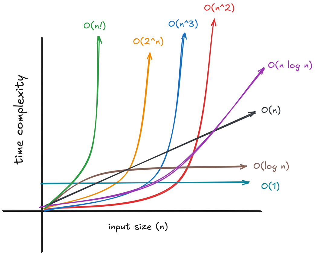
Compare the flat O(1) line with curves that rise as input size increases. section 1.3.1