Cubic polynomial

As explained in Geometry for Programmers

A cubic equation is an equation containing a polynomial expression of degree three in its variable.

A cubic polynomial is a third-degree polynomial: its highest nonzero power is x³. In canonical form, it is ax³ + bx² + cx + d, with a nonzero. Coefficients may be zero, one, or negative; for example, C(x) = x³ - 2x² + 4 has no x term, but is still cubic. section 6.1 section 6.1.1

Writing the cubic as ax³ + bx² + cx + d = 0 turns root finding into a geometric question: roots are the places where its graph meets the x-axis. A cubic has one, two, or three such roots; a double root occurs when the graph touches the axis rather than crossing it. A monic cubic can also be written as (x - r₁)(x - r₂)(x - r₃), where each r makes the polynomial zero. section 6.1 section 6.1.1

Figure 6.3 A cubic polynomial may have one, two, or three roots.

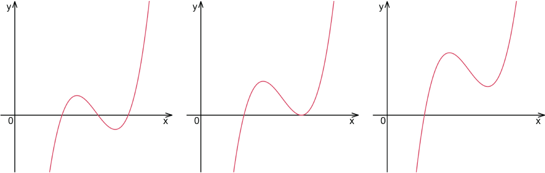
Use the graph to connect algebraic roots with crossings and touches of the x-axis. section 6.1.1

Several forms make the same cubic useful for different jobs:

• Use canonical form, ax³ + bx² + cx + d, when inspecting degree and coefficients. section 6.1
• Use Horner’s form, ((ax + b)x + c)x + d, to evaluate efficiently: it reduces the example calculation from six multiplications to three. section 6.1
• Use factored form when roots are known and zeros matter. section 6.1
• Use parametric cubic pieces x(t) and y(t) when a curve must meet endpoint positions and tangent directions. section 11.4.2 section 12.4.4

Differentiation lowers a cubic to a quadratic. For P(x) = x³ - x² - 2x + 1, P′(x) = 3x² - 2x - 2. Roots of the derivative identify horizontal turning candidates: when the derivative changes from negative to positive or positive to negative, the cubic has a local minimum or maximum. A derivative root that only touches its own axis need not produce an extremum in the cubic. section 6.1.2 section 5.1.2

Smoothing a sampled contour

Replace a straight contour segment with a cubic parameterized over t from 0 to 1. Solve separate cubic equations for x(t) and y(t) so the curve starts and ends at the segment’s endpoints and matches tangent vectors there. Gradients can supply tangent directions, but oversized tangent vectors can make the cubic loop; normalizing them preserves smoothness while avoiding those loops. section 12.4.4 section 11.4.2

How Geometry for Programmers covers it

How deep it goes

Develops canonical, factored, and Horner forms; derivatives; and endpoint-and-tangent fitting equations for parametric cubics.

Examples

Uses x³ - 2x² + 4, x³ - x² - 2x + 1, root-intersection plots, and smoothed contours fitted from SDF data.

What it assumes

Builds from polynomial notation and elementary differentiation rules for powers, constants, and sums.

What you can do after

Build it from scratch, fit endpoint-and-tangent-constrained cubic curve pieces and prevent loops by normalizing tangents.

How it connects

Connects polynomial roots, Horner’s method, derivatives, local extrema, tangent vectors, parametric curves, and signed distance fields.

liveBookmanning.com

Read Geometry for Programmers on liveBook Get the book at manning.com

Related concepts

• polynomial functionkind of · A polynomial function is a function expressible as a finite sum of constant multiples of nonnegative integer powers of one or more variables.
• linear systemproduced by · A linear system is a set of linear relationships among variables, commonly expressed as simultaneous equations or a linear transformation, for which superposition applies.
• Bézier curveequivalent to · A Bézier curve is a parametric curve whose shape is determined by control points through Bernstein basis functions.

This explainer was generated by Manning's knowledge graph from the text of Geometry for Programmers. The section links point to the parts of the book it draws on.