Cumulative probability totals the probability that a random variable is less than or equal to a specified value: F(x) = P(X ≤ x). For discrete outcomes, sum the probabilities of every value up to x; for continuous variables, obtain the corresponding area under the probability density function. section 2.4.3 section 2.3.3
Use these properties to calculate and interpret cumulative probabilities:
- Treat the cumulative probability as nondecreasing: increasing x can only increase or preserve the total, never reduce it. section 2.4.3
- Keep values between 0 and 1; the final cumulative probability reaches 1 when all possible outcomes have been included. section 2.4.3
- Find an interval probability with P(a < X ≤ b) = F(b) − F(a). section 2.3.3
- For simulation, convert cumulative totals into random-number intervals so each generated number maps to an outcome with the intended probability. section 9.2
Dice and absenteeism examples
For two six-sided dice, P(X ≤ 4) adds the probabilities of 2, 3, and 4: 0.0278 + 0.0556 + 0.0833 = 0.167, or 16.7%. For a Poisson model with λ = 2, the cumulative probability of at most two absentees is 13.53% + 27.07% + 27.07% = 67.67%. section 2.4.3 section 9.3.2
>>> cumulative_probabilities = \
>>>     poisson.cdf(k_values, lam)     #1
>>> cumulative_percentage = \
>>>  np.round(cumulative_probabilities * 100, 2)     #2
>>> poisson_table = pd.DataFrame({'k': k_values, \
>>>                     'Probability (%)': probabilities_percentage, \
>>>                     'Cumulative Probability (%)': \
>>>                 cumulative_percentage})  #3
>>> print(poisson_table)    #4
   k  Probability (%)  Cumulative Probability (%)
0  0            13.53                       13.53
1  1            27.07                       40.60
2  2            27.07                       67.67
3  3            18.04                       85.71
4  4             9.02                       94.73
5  5             3.61                       98.34
6  6             1.20                       99.55
7  7             0.34                       99.89
8  8             0.09                       99.98
Inspect the Python listing to calculate Poisson cumulative probabilities with poisson.cdf(), round percentages, and assemble a pandas table. section 9.3.2
Figure 2.5 The CDF for rolling a pair of six-sided dice. The shape of the distribution resembles a two-dimensional flight of stairs in which the horizontal line segments represent consecutive values for x and the vertical lines represent their respective probabilities.
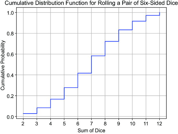
Use the step-function figure to see how each discrete probability raises the cumulative total at successive outcomes. section 2.4.3
