A distribution function maps outcomes of a random variable to probability values. For a coin-flip variable X, P(X = 1) = 0.51 assigns heads its probability; P(X) denotes the distribution over all outcomes. section 2.1.2
For a finite discrete variable, a table lists each outcome and its probability. Continuous variables instead use a probability density function, whose values describe relative likelihood and integrate over intervals to produce probabilities. section 2.1.2 section 2.1.7
Useful distinctions make the representation operational:
- Categorical distributions represent discrete categories; Bernoulli distributions have two outcomes, and discrete uniform distributions assign equal probabilities. section 2.1.7
- Canonical distribution classes become concrete when parameters such as location, scale, rate, or shape are supplied. section 2.1.7
- Joint distributions map combinations of outcomes, while conditional distributions describe how one variable’s distribution changes given another. section 2.5 section 2.1.8
Representing and evaluating a discrete distribution
A three-outcome variable can assign probabilities 0.45, 0.30, and 0.25 to outcomes 1, 2, and 3. In pgmpy, DiscreteFactor stores this table; in Pyro, Bernoulli(probs=0.4) represents a two-outcome distribution, and log_prob can recover the probability of outcome 1. section 2.1.2 section 2.1.7
Figure 2.3 A simple tabular representation of a discrete distribution
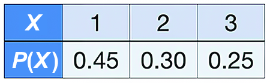
Use the tabular representation to inspect how discrete outcomes, states, and probability values form a complete distribution. section 2.1.2
Figure 2.11 Visualization of a discrete probability distribution. The outcomes in the distribution are on the horizontal axis, and probability is on the vertical axis.
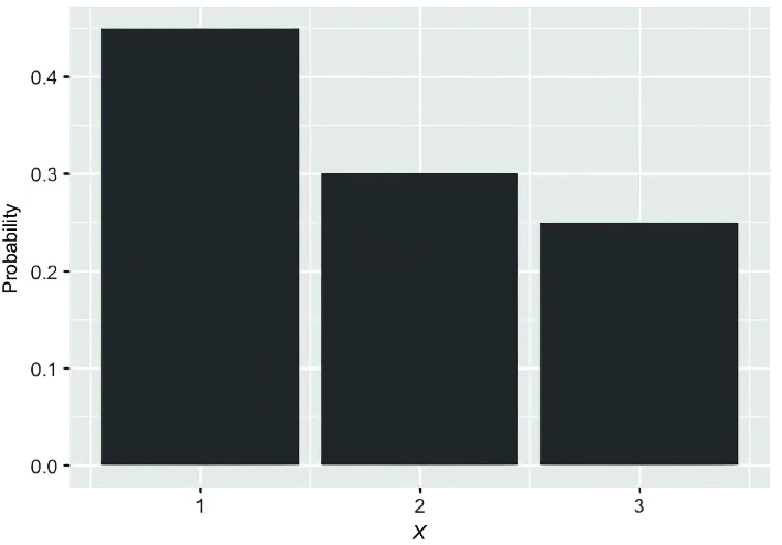
Use the bar plot to connect the outcome axis with the probability axis and distinguish distribution visualization from a histogram. section 2.1.8
