Suppose you have a fixed cloud budget and several server instances, each with a cost and a throughput value. Which combination gives the most throughput? Trying every include-or-skip combination becomes expensive as the list grows. Dynamic programming avoids repeating the same smaller calculations: record the best answer for each smaller budget and set of available instances, then reuse it. section 7.0 section 7.1
For 0/1 knapsack, build the answer from small cases upward:
- Make a table with rows for how many items may be used and columns for capacities from zero through the budget. With no items or no capacity, the best value is zero. section 7.1
- For each cell, ask: does the current item fit? If not, copy the answer from the row above. section 7.1
- If it fits, compare skipping it with taking its value plus the previous row’s answer for the remaining capacity. Store the larger result. Looking at the previous row keeps the choice strictly 0/1. section 7.1
Figure 7.3 Visualization of the math used to evaluate cell T[2, 3] (circled in green) on the second row (w2 = 2, v2 = 3). The algorithm resolves a binary choice by executing a maximum value comparison between two paths. The exclusion path inherits the value directly above (T[1, 3] = 2). The active inclusion path accepts the new instance's throughput value (v2 = 3, highlighted in the red solid box) and subtracts its weight from the current capacity (3 - 2 = 1), forcing a pointer lookup to the previous row at column 1 (T[1, 1] = 2, highlighted by the red dotted circle). The combined value of 5 outperforms the exclusion path, updating the cell state.
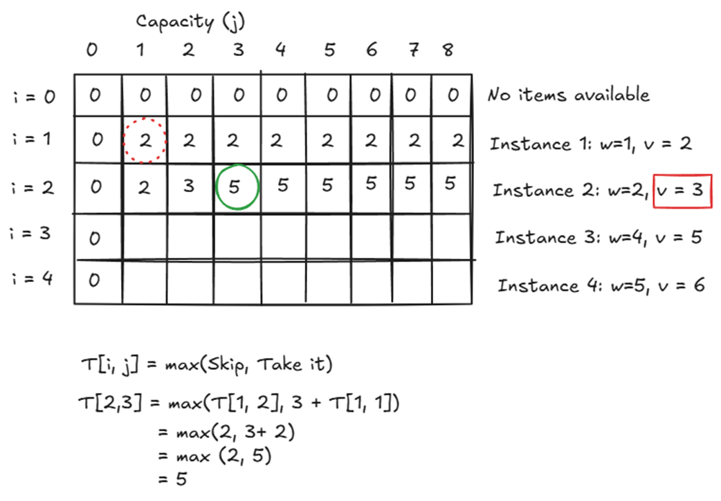
Follow the two lookups for capacity 3 and the second item: skipping gives 2; taking gives 3 plus the earlier answer of 2, so the cell becomes 5. section 7.1
Finish a small capacity plan
Four instances cost 1, 2, 4, and 5 credits and provide values 2, 3, 5, and 6. At capacity 8, the final choice compares skipping the fourth instance, worth 10, with taking it and using the best value at the remaining capacity of 3: 6 + 5 = 11. The stored answer is 11. section 7.1
This table takes O(n × W) time and O(n × W) space for n items and capacity W. A one-dimensional array can reduce memory because each choice needs values from the preceding row, but the full table makes those dependencies easier to see. For divisible goods, fractional knapsack instead permits a greedy value-per-weight approach; do not assume that approach works when items cannot be split. section 7.3
The same habit—save answers to smaller cases and use them to improve larger ones—also appears in Floyd–Warshall. Its distance matrix compares the best known route between two vertices with a route through a newly considered intermediate vertex. Here the stored result is a shortest distance, not a maximum item value. section 9.1