Dynamic quantization adapts activation scales during inference instead of fixing them with a calibration dataset. It is useful when input distributions vary, but runtime scale computation has a cost. Dynamic-range deployments can also store weights in reduced precision; the actual activation and compute dtypes depend on the runtime and graph. section 3.3 section 11.2.1
For symmetric INT8 activation quantization, find the input tensor’s maximum absolute value and divide it by 127 to obtain the scale. Divide each value by that scale, round, and clamp to −127 through 127. Return the scale with the quantized tensor so values can later be reconstructed by multiplying by the scale. An all-zero tensor can use a scale of 1. section 3.3
Listing 3.19 Dynamic quantizer
class DynamicQuantizer:
    def __init__(self, bits=8, symmetric=True):
        self.q_max = (1 << (bits - 1)) - 1 if symmetric else (1 << bits) - 1
        self.q_min = -self.q_max if symmetric else 0
        self.symmetric = symmetric

    def quantize(self, tensor):
        if self.symmetric:
            abs_max = tensor.abs().max().item()
            scale = abs_max / self.q_max if abs_max > 0 else 1.0
            zero_point = 0
        else:
            min_val, max_val = tensor.min().item(), tensor.max().item()
            scale = (max_val - min_val) / (self.q_max - self.q_min)
            zero_point = int(round(self.q_min - min_val / scale))

        q_tensor = torch.clamp(
            torch.round(tensor / scale + zero_point),
            self.q_min, self.q_max
        ).to(torch.int8)

        return q_tensor, scale, zero_point                        #A
The quantizer computes scales at runtime and returns them with the quantized tensor. section 3.3
Changing input distributions
With a static scale fixed at 0.0488, a wide synthetic input produced MSE of 1.799070; recomputing the scale dynamically reduced MSE to 0.001597, about 1,126× lower. On typical inputs matching calibration, the improvement was only 1.10×. These are comparisons for the measured inputs, not guaranteed gains. section 3.3
A single dynamic scale still exposes typical values to outlier-driven resolution loss. In one BERT activation sample, the maximum was 25.8 while the median magnitude was 1.93. Scaling to the maximum gave the median roughly nine quantization levels; scaling to the 99th percentile gave roughly 51 but clipped the largest values. section 3.3
Per-token dynamic quantization computes a separate scale across each token’s hidden dimension. It uses more scale storage than per-tensor quantization but can better accommodate tokens with different ranges. In one synthetic comparison, per-token MSE was 0.000099 versus 0.001629 for dynamic per-tensor quantization, a 16.46× reduction. section 3.3
TFLite dynamic-range conversion uses Optimize.DEFAULT without a representative dataset. Verify the converted graph rather than assuming this produces integer activation math: in one EfficientNet-Lite0 graph, weights were INT8 but activations remained FP32, and kernels dequantized weights for FP32 matrix multiplication. Per-operation dequantization costs latency relative to INT8 on that path. section 11.2 section 11.2.1
Figure 11.6 TFLite per-tensor dtype map across the four converter paths. Each bar is the tensor count per dtype in the produced flatbuffer. FP32 has 161 float32 tensors plus one int32 (a shape constant). Dynamic-range has 60 int8 (weights), 129 float32 (activations and biases), 15 int32. The converter has quantized only the weights and left every activation tensor in FP32. INT8 has 111 int8, 51 int32, zero float32. The integer pipeline is end-to-end, no float remains in the graph. INT16×8 has 62 int16 activations, 50 int8 weights, 50 int64 (zero-points and scales held at higher precision), 4 int32, and two float32 tensors, the input and output. The two float fallbacks are by design (the operator at the I/O boundary always materializes its tensor in the inference-input dtype the API was constructed with), but they are also why the experimental supported-ops set is called experimental.
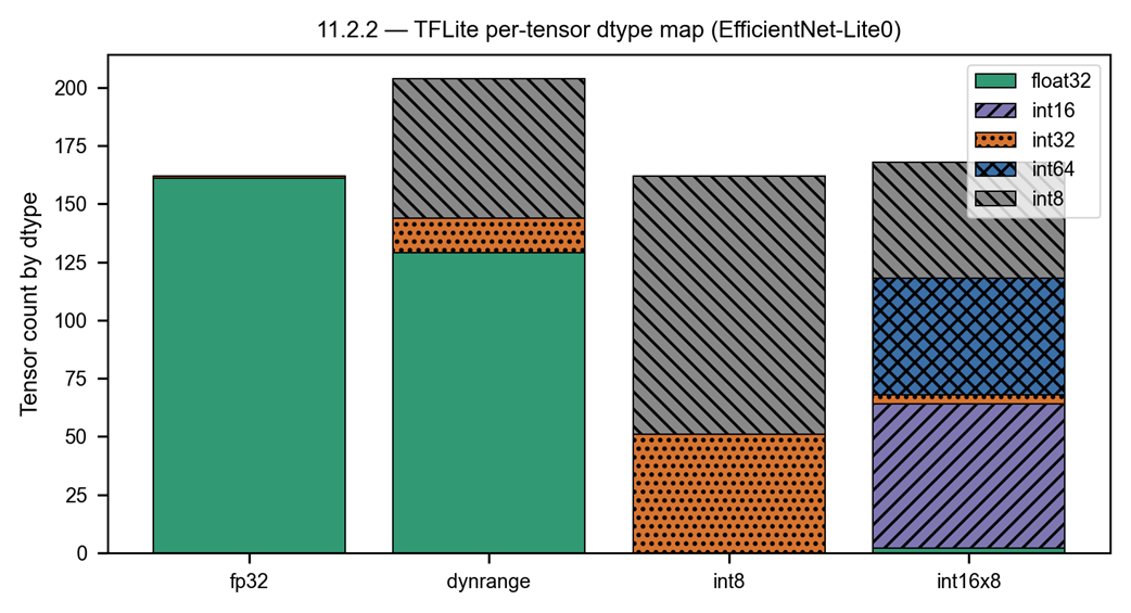
The dtype map distinguishes weight compression from an end-to-end integer graph. section 11.2.1
TFLite deployment checks
On BERT-base SST-2, dynamic-range conversion reduced size from 416.65 MB to 105.85 MB with accuracy unchanged at 92.43% over 872 validation samples. Conversion required concrete input shapes in this path. Inspect tensor dtypes with tf.lite.Interpreter.get_tensor_details() and measure accuracy and latency on the intended runtime and device. section 6.3 section 11.2.1