An elasticity plot is a demand-specific error-analysis tool for pricing models. It shows how predicted sales change as price changes, testing the core expectation that higher prices generally reduce demand. It is a specialized partial dependence plot and can also be viewed as residual analysis for a pricing system. section 9.2.6
Build the curve in one of two practical ways:
- Use training data: select a SKU’s sales history, predict sales for each historical row, pair each prediction with its actual historical price, and plot price against predicted sales. section 9.2.6
- Use mixed synthetic and real data: take the SKU’s latest price, vary it from −20% to +20%, recalculate price-based features, predict sales for every variation, and plot the results. section 9.2.6
- Expect an inverse, reasonably monotonic relationship; an opposite, noisy, or nonmonotonic curve signals limited price variation, stochastic demand, confounding promotions or seasonality, or a model that misses the case. section 9.2.6
Validating a retail model
Before deploying a new demand model, compare elasticity curves for individual goods and confirm with stakeholders whether those goods should be elastic. If the curves fail the expected relationship, apply isotonic-regression postprocessing as a fast, ad hoc calibration option, or improve modeling, features, and preprocessing for a slower generic solution. section 9.4.1
Figure 9.18 Theoretical example of elastic demand
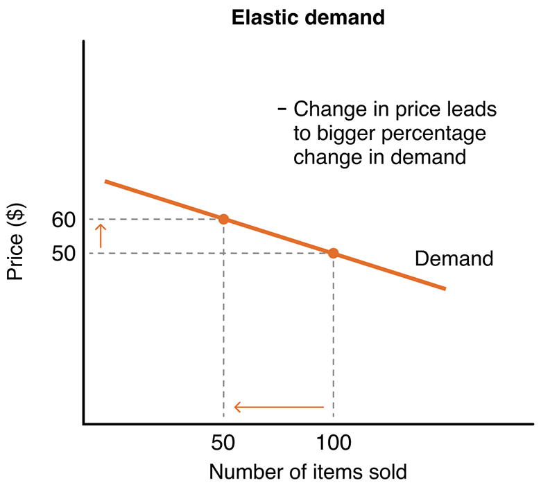
Use the theoretical elastic-demand figure to contrast the expected response shape with observed SKU curves. section 9.2.6
Figure 9.19 Theoretical example of inelastic demand
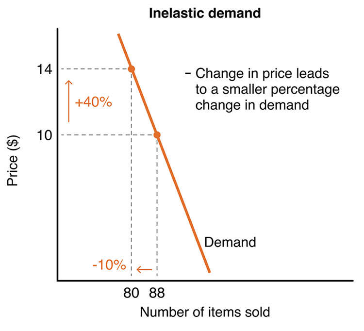
Use the theoretical inelastic-demand figure when comparing goods whose predicted sales respond weakly to price changes. section 9.2.6
