A fuel-ordering decision may affect whether a gas station runs out days later. An eligibility trace helps assign credit or blame for that later outcome to earlier decisions, rather than only the most recent one. section 6.5 section 6.6
An eligibility trace is a short-term record of how eligible a state or state–action pair is to receive an update from the current temporal-difference (TD) error. Recent visits have larger traces; older traces decay. Repeated visits can also increase a pair’s eligibility, reflecting both recency and frequency. section 6.5
The backward-view approach updates estimates online, without waiting for future rewards:
- Record visits in traces, with recent or frequent visits carrying more eligibility. section 6.5
- Use the current TD error to update eligible estimates, weighted by their traces. section 6.5 section 6.7
- Let traces decay so that older visits gradually receive less credit. section 6.5
The parameter λ controls how far back credit is assigned. It gives a tunable spectrum between one-step TD at λ = 0 and Monte Carlo at λ = 1. The backward view uses traces to achieve online updates, whereas the forward view considers returns involving future rewards. section 6.5 section 6.7
Figure 6.8 Update mechanism of temporal difference learning with eligibility traces.
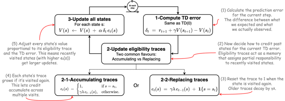
Follow how a TD error updates earlier visits through their eligibility traces. section 6.5
Fuel purchase scheduling
A station chooses whether to order fuel while demand and delivery times are uncertain. A later stockout penalty can inform earlier ordering decisions through their traces. SARSA(λ) uses this idea with on-policy learning; Watkins’s Q(λ) adapts it to off-policy learning by resetting traces when a non-greedy action is taken. section 6.6 section 6.7
