Elliptic curve point addition combines two points P₁=(x₁,y₁) and P₂=(x₂,y₂) on an ordinary curve into R=P₁+P₂=(x₃,y₃), another point on that curve. Geometrically, draw a line through the inputs, find its other intersection with the curve, then take that point’s negative. Over finite fields, the same addition rules support the arithmetic used later for point multiplication. section 3.1.3 section 3.6 section 3.1.2
Use the curve form y²=x³+a₄x+a₆. A single slope formula handles both distinct inputs and doubling P₁=P₂: λ=(x₁²+x₁x₂+x₂²+a₄)/(y₁+y₂). Then compute x₃=λ²−x₁−x₂ and y₃=λ(x₁−x₃)−y₁. Using one form for tangents and ordinary additions avoids selecting separate formulas that could reveal secret-key information through power analysis. section 3.1.3 section 3.6
Figure 3.4 Adding a point to itself
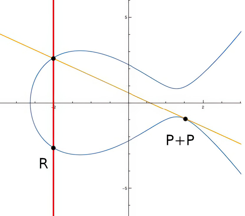
The tangent picture makes doubling concrete: adding a point to itself follows the same group law, with the tangent replacing a line through two distinct points. section 3.1.3
An implementation-oriented addition routine proceeds as follows:
- Treat the point at infinity 0 as the identity: if either input is 0, return the other input unchanged. section 3.2.2 section 3.6
- Compute the numerator and denominator for λ with modular arithmetic before dividing. section 3.2.2
- When y₁+y₂ is zero, test x₁=x₂. If both conditions hold, the points are negatives and the result is 0; otherwise use (y₂−y₁)/(x₂−x₁) for the slope. section 3.2.2
- Calculate x₃ and y₃ in a temporary point, then copy it to the result so an input is not overwritten during calculation. section 3.2.2
- Clean up temporary arithmetic objects after producing the result. section 3.2.2
The inverse-point case
Suppose two non-infinity points have opposite y-values and the same x-value. Their y-values sum to zero, so the unified slope denominator cannot be used. The matching x-values identify the points as inverses, and their sum is the point at infinity rather than an ordinary coordinate pair. section 3.2.2 section 3.6
The same equations extend to field-extension curves: replace each coordinate and curve coefficient with a polynomial reduced modulo an irreducible polynomial. The control flow remains the same—identity checks, exceptional slope handling, coordinate calculation, and cleanup—but polynomial values require separate initialization and removal. section 13.2.5 section 13.0
Point addition is the core subroutine for double-and-add point multiplication. Reusing the same routine for both doubling and addition also strengthens the implementation against distinctions between those operations. section 3.2 section 3.6