An error surface maps model weight values to prediction error. Picture a landscape: each point represents one set of weights, and lower locations represent predictions with less error. For a single training example, the minimum is the weight setting closest to zero error. section 5.3
For a complete training set, the surface uses aggregate error rather than one example’s error. Mean squared error can form the vertical axis; the lowest location represents weights that fit the training set as well as possible. section 5.3
The surface provides a mental model for training behavior:
- On a convex surface, gradient descent repeatedly follows the downward direction toward the minimum. section 5.3.1
- On a nonconvex surface, pits and divots can create local minima, where training stops even though a lower global minimum may exist. section 5.3.1
- With many weights, visualization becomes impractical; plotting error or a related metric over training time provides a more useful signal. section 5.3.1
- Stochastic gradient descent reshuffles training examples between passes, changing the path across the surface and potentially helping avoid traps. section 5.3.2
Skiing toward lower error
Imagine skiing down a mountain while adjusting model weights. At each step, the gradient indicates a downhill direction. A smooth bowl makes the route straightforward; scattered pits can trap the skier at local minima. Shuffling examples changes the route, while short updates reduce the risk of following one sample’s estimate too far. section 5.3.1 section 5.3.2
Figure 5.6 Convex error curve
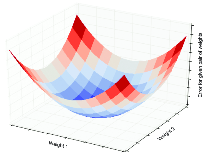
Use the convex curve to visualize how two weight dimensions and error form a bowl-shaped landscape. section 5.3
Figure 5.7 Nonconvex error curve
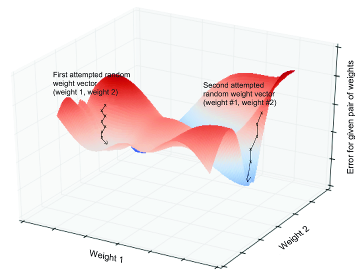
Use the nonconvex curve to visualize pits, local minima, and dependence on the starting weights. section 5.3.1
