Marginal likelihood

As explained in Bayesian Optimization in Action

A marginal likelihood is the probability or density of observed data after integrating over latent variables or model parameters.

Marginal likelihood measures how well a Gaussian process explains its training data under particular model settings. Comparing likelihoods turns modeling choices into a practical selection problem: prefer the mean or covariance parameters that assign higher likelihood to the observations. section 3.3.2

For a Gaussian process, the marginal log likelihood is computed from the model and its hyperparameters. Maximizing it seeks the settings that explain the observed data best; gradient descent performs this search by repeatedly updating the parameters toward higher likelihood. section 3.3.2 section 3.4.1

Choosing a constant mean

Suppose observations come from an exclusively positive function. Compare Gaussian processes with constant means of 0 and 2. The model reverting to 2 receives the higher likelihood because that mean explains the training observations better. In code, GPyTorch constructs an ExactMarginalLogLikelihood, minimizes its negative value with Adam, and tracks convergence of the mean and loss. section 3.3.2

The same objective selects covariance behavior. Optimizing the length scale and output scale can produce a smoother GP with a wider prediction range; for a three-point dataset, gradient descent found values of roughly 1.3 and 2.1. section 3.4.1

Figure 3.6 GP predictions, given two different constant mean functions. The value 2 gives a higher likelihood value than the value 0, indicating the former mean function is a better fit than the latter.

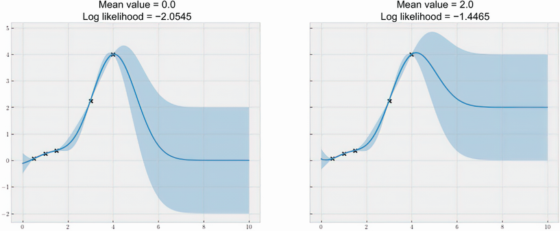
Compare the two GP predictions to see how the higher-likelihood constant mean better fits the training observations. section 3.3.2

How Bayesian Optimization in Action covers it

How deep it goes

Defines likelihood-based fitting, demonstrates parameter comparison, and gives an optimization loop without deriving the probability calculation.

Examples

Compares constant means of 0 and 2 and tunes length and output scales on a three-point training dataset.

What it assumes

Assumes Gaussian-process models and basic gradient descent, while illustrating likelihood optimization through concrete parameter choices.

What you can do after

Apply it via GPyTorch and Adam to optimize Gaussian-process mean or covariance parameters.

How it connects

Connects Gaussian processes, mean functions, covariance functions, hyperparameters, kernels, and gradient descent.

liveBookmanning.com

Read Bayesian Optimization in Action on liveBook Get the book at manning.com

Related concepts

• evidence lower boundused by · The evidence lower bound is a variational objective that lower-bounds a model’s log marginal likelihood and is optimized to approximate the posterior distribution.
• regularizationequivalent to · Regularization is a modeling technique that constrains or penalizes solutions during fitting or optimization to discourage undesirable complexity or behavior and improve generalization or estimation.
• marginal probabilityequivalent to · A marginal probability or distribution describes a variable or event without conditioning on other variables, obtained from a joint distribution by summing or integrating over them.
• language modelmeasures · A language model is a computational model that represents patterns in linguistic tokens to estimate sequence probabilities and predict or generate language from context.

This explainer was generated by Manning's knowledge graph from the text of Bayesian Optimization in Action. The section links point to the parts of the book it draws on.