A feature space is the multidimensional input space of a machine-learning problem. Each scalar feature supplies one coordinate axis, and one complete input vector is a single point. Its dimension is the number of input variables: hardness and sharpness make a two-dimensional space, while realistic inputs may require hundreds, thousands, or more dimensions. Thinking in points and coordinates gives a geometric view of what a model receives. section 1.4 section 7.2.2
A model maps points from feature space to points in an output space. For classification, this mapping should make classes easier to distinguish: points that belong to different classes are sent to separate output clusters. Equivalently, a classifier partitions feature space with a decision boundary. An unknown input is classified by the region, or side of the boundary, in which its point lies. section 1.4 section 3.8
Hardness and sharpness
Let x = (x0, x1), where x0 measures hardness and x1 measures sharpness. Every object becomes a point in a 2D feature space. A simple threat score is its signed distance from the separator x0 + x1 = 1: y = (x0 + x1 − 1)/√2. The sign of y identifies which side of the line the point occupies. This turns two measured properties into a geometric classification rule. section 1.4
Figure 1.2 2D input point space for the cat brain model. The bottom-left corner shows objects with low hardness and low sharpness objects (–), while the top-right corner shows objects with high hardness and high sharpness (+). Intermediate values are near the diagonal ($).
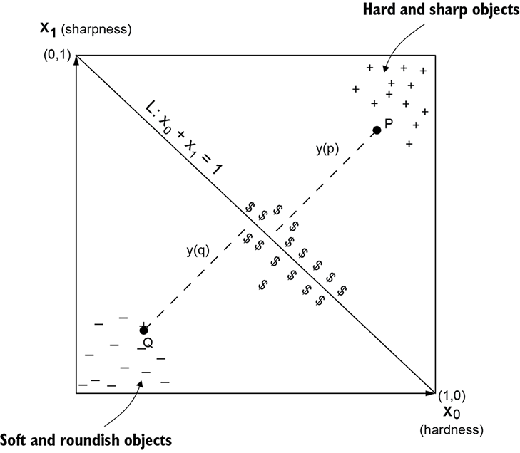
Inspect the two axes as features and the diagonal as a separator: low-hardness, low-sharpness points lie apart from high-value points, while intermediate cases sit near the boundary. section 1.4
Feature spaces need not be easy to visualize. An image can be represented by a vector with one scalar variable per pixel; a 224 × 224 image therefore lies in a 50,176-dimensional input space, and each particular image is one point. A face classifier maps that point to 0 or 1. In document representations, each vocabulary word can define a dimension, with word frequency as its coordinate value. Such vectors are sparse because absent words need not be stored explicitly. section 7.2.2 section 4.1
The geometry also reveals structure in high-dimensional data. If two document terms tend to occur together, their coordinates vary together; projected onto those two axes, document points lie roughly along the line x = y. More generally, classification training seeks a boundary that separates labeled point clusters. A simple problem may use a hyperplane, whereas classes that cannot be separated by a line, plane, or hyperplane require a curved boundary and a more expressive model. section 4.1 section 3.8 section 1.4
Figure 4.1 Document descriptor space. Each word in the vocabulary corresponds to a separate dimension. Dots show projections of document feature vectors on the plane formed by the axes corresponding to the terms gun and violence.
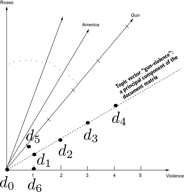
Use the document-space projection to see how correlated word-frequency features constrain points to a lower-dimensional pattern within a very large feature space. section 4.1
