Need derivatives for several outputs without building a full Jacobian? Forward-mode autodiff propagates derivative information alongside ordinary values during one forward evaluation. In JAX, jvp() exposes this calculation directly, while jacfwd() repeats it to construct a Jacobian. section 4.3.2 section 4.4
Each intermediate value travels as a pair: a primal value and a tangent derivative. Applying the chain rule to these pairs is the dual-numbers view of forward mode. A single pass produces the function output and its derivative in the chosen input direction. section 4.3.2 section 4.3.1
A directional derivative with jvp()
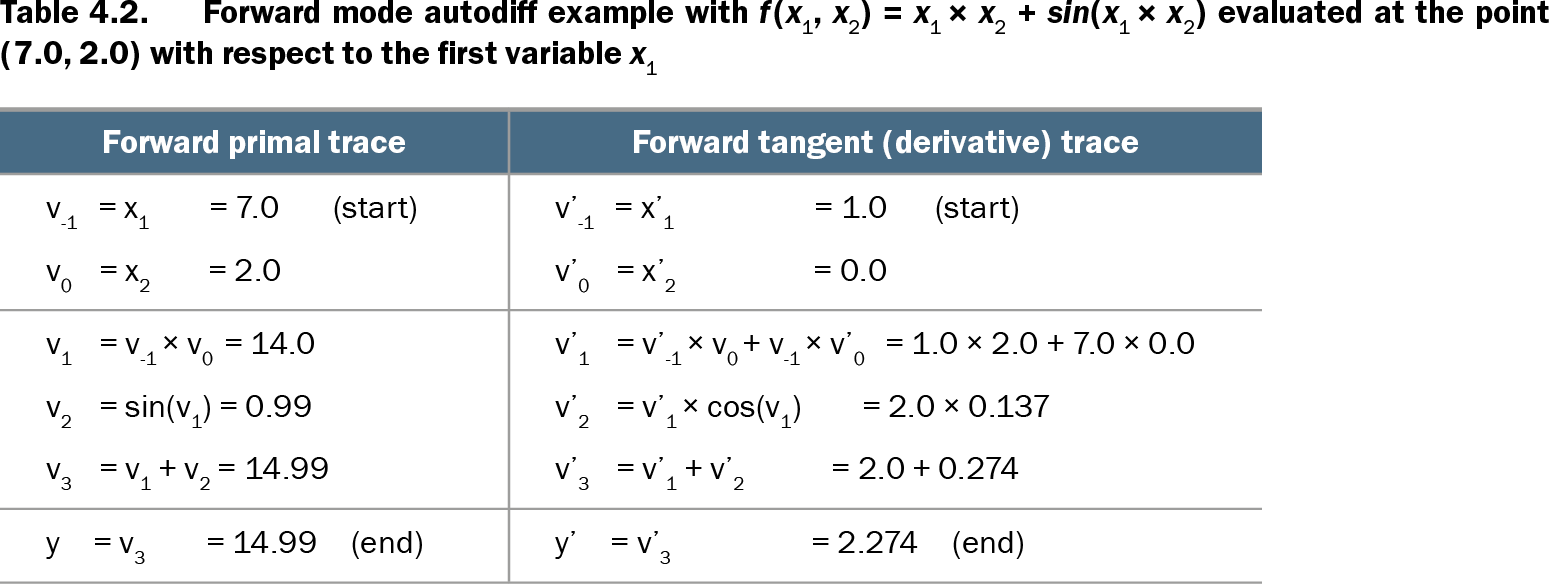
For f(x1, x2) = x1 × x2 + sin(x1 × x2), evaluate at (7.0, 2.0) and seed the first input direction: p, t = jax.jvp(f, (7.0, 2.0), (1.0, 0.0)). The primal result is approximately 14.990607, and the tangent is approximately 2.2734745, the derivative with respect to x1. Changing the tangent seed changes the direction being differentiated. section 4.3.2
Forward mode computes derivatives for every output with respect to one input direction in a pass. Consequently, it suits tall Jacobians: functions with many outputs and relatively few inputs. A full Jacobian requires one forward evaluation per input variable; jacfwd() automates that process. section 4.3.2 section 4.2.5
Use forward mode when:
- You need a Jacobian-vector product without materializing the Jacobian. section 4.4
- Your function has significantly more outputs than inputs, or its Jacobian is tall or near-square. section 4.3.2 section 4.2.5
Forward mode is the counterpart to reverse mode. Reverse mode first records the computation and then propagates adjoints backward, making it preferable when many inputs feed a small number of outputs, as in typical loss gradients. section 4.3.3 section 4.4
Table 4.2. Forward mode autodiff example with f(x1, x2) = x1 × x2 + sin(x1 × x2) evaluated at the point (7.0, 2.0) with respect to the first variable x1 (view table figure)
| Forward primal trace |
Forward tangent (derivative) trace |
|---|---|
| v−1 = x1 = 7.0 (start) v0 = x2 = 2.0 |
v’−1 = x’1 = 1.0 (start) v’0 = x’2 = 0.0 |
| v1 = v−1 × v0 = 14.0 v2 = sin(v1) = 0.99 v3 = v1 + v2 = 14.99 |
v’1 = v’−1 × v0 + v−1 × v’0 = 1.0 × 2.0 + 7.0 × 0.0 v’2 = v’1 × cos(v1) = 2.0 × 0.137 v’3 = v’1 + v’2 = 2.0 + 0.274 |
| y = v3 = 14.99 (end) |
y’ = v’3 = 2.274 (end) |
Follow the primal and tangent traces for x1 × x2 + sin(x1 × x2), including the intermediate chain-rule calculations that produce the final derivative. section 4.3.2