A causal model may fit observed data yet leave uncertainty about its parameters. Bayesian estimation treats those parameters as random variables: assign each a prior distribution, then condition on observed data to obtain a posterior distribution. Rather than committing only to one fitted value, posterior samples can carry parameter uncertainty into predictions and causal inferences. If the model has latent variables, inference can target them jointly with the parameters. section 2.3.4
For a causal-effect estimate, keep estimation distinct from intervention:
- Estimate the causal graphical model’s parameter distributions from data, with a prior for each parameter vector. section 11.6.3
- Transform the fitted model to represent the intervention, then run probabilistic inference on the transformed model. The effect calculation can depend on samples from the parameter posterior. section 11.6.3 section 11.6
Categorical probabilities: a tractable exception
For a conditional probability table, maximum likelihood uses proportions of observed counts. A Dirichlet prior instead combines prior parameters with those counts. Because the prior is conjugate to the categorical model, the posterior is also Dirichlet and its parameters can be calculated directly. pgmpy’s BayesianEstimator uses this route to return point estimates; those output values should not be mistaken for posterior samples. More general Bayesian estimation may require sampling algorithms or variational inference. section 3.1.9
Listing 3.5 Bayesian point estimation with a Dirichlet conjugate prior
from pgmpy.estimators import BayesianEstimator     #1
model.fit(
    data,
    estimator=BayesianEstimator,    #2
    prior_type="dirichlet",
    pseudo_counts=1    #3
)
causal_markov_kernels = model.get_cpds()      #4
cmk_T = causal_markov_kernels[-1]     #4
print(cmk_T)  #4
The pgmpy listing shows the concrete point-estimation setup: select BayesianEstimator, specify a Dirichlet prior and pseudo-counts, then inspect the fitted conditional probability tables. section 3.1.9
Figure 11.15 A plate model of the causal DAG with new nodes representing parameters associated with each causal Markov kernel. There is a single plate with N identical and independent observations in the training data. θ corresponds to parameters, which are outside the plate, because the parameters are the same for each of the N data points.
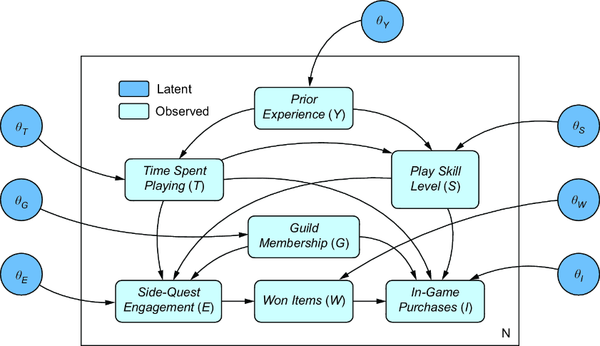
The plate diagram separates shared parameter nodes, outside the observation plate, from the repeated data points they help model. section 11.6.3

