Gaussian mutation changes a real-valued gene by adding a random perturbation sampled from a Gaussian distribution with mean zero. The standard deviation σ sets the mutation step: larger values make broader moves, while smaller values make gentler adjustments. These perturbations preserve population diversity and can help a real-valued genetic algorithm escape local optima. section 8.2.2
Use Gaussian mutation by following this practical sequence:
- Select a continuous gene, such as one coefficient in a polynomial-fitting chromosome. section 8.2.2
- Sample a zero-mean Gaussian random value using the chosen σ. section 8.2.2
- Add the sampled value to the gene, then evaluate whether the altered individual improves the objective. section 8.2.2
- Tune σ to balance exploration and exploitation: larger steps search more widely, whereas smaller steps refine nearby solutions. section 8.5
Polynomial curve fitting
Represent a third-order polynomial with four genes, a, b, c, and d, and use a real-valued genetic algorithm to minimize mean squared error against sampled x and y values. Gaussian mutation can perturb any coefficient during the search, producing a nearby candidate polynomial without replacing the coefficient wholesale. The same setting supports comparison with Cauchy, boundary, and polynomial mutation. section 8.2.2
Table 8.2 Curve-fitting problem data (view table figure)
| x |
0 |
1.25 |
2.5 |
3.75 |
5 |
| y |
1 |
5.22 |
23.5 |
79.28 |
196 |
Inspect the sampled curve-fitting data used to motivate mutation operators and evaluate candidate polynomial coefficients. section 8.2.2
Gaussian mutation need not use a fixed step size. A deterministic schedule can reduce σ from 1 at the start to 0.1 by the final generation, shifting from exploration toward exploitation. An adaptive strategy can instead increase variance when more than one mutation succeeds in five trials, following Rechenberg’s 1/5 success rule; otherwise, it decreases variance. section 8.5
Figure 8.14 Rechenberg’s 1/5 success rule. Following this rule, the Gaussian distribution’s standard deviation is updated by a constant. The higher the standard deviation, the higher the value of x (i.e., larger step size), the higher the deviation from the current solution (more exploration), and vice versa.
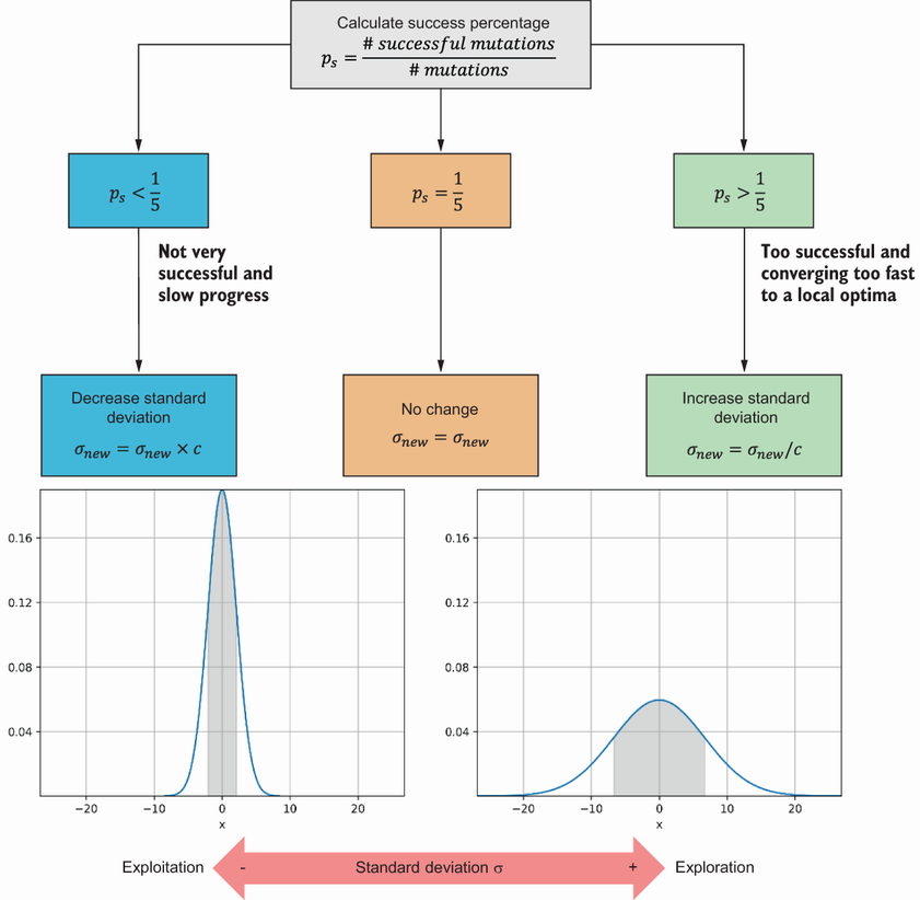
Use the figure to relate standard deviation, mutation step size, distance from the current solution, and exploration. section 8.5

