Suppose you are estimating how much a house’s price changes with each additional square foot. Before looking at sale prices, you might expect about $100 per square foot—but be far from certain. A Gaussian prior, also called a normal prior, puts that starting belief into a probability distribution for the unknown slope. section 3.12
A normal prior is written 𝒩(μ, σ²). Its mean μ is the most likely value; its standard deviation σ controls the spread. For the house-price slope, 𝒩(100, 100²) centers the prior at 100 while leaving considerable room for other values. Roughly 95% of its probability lies between μ − 2σ and μ + 2σ: here, about −100 to 300. section 3.12
Figure 3.4 The prior distribution of the slope 𝑚 in the linear regression model, which gives the highest probability to the value 100 but there’s a high level of uncertainty in this value, quantified by the large spread of the distribution.
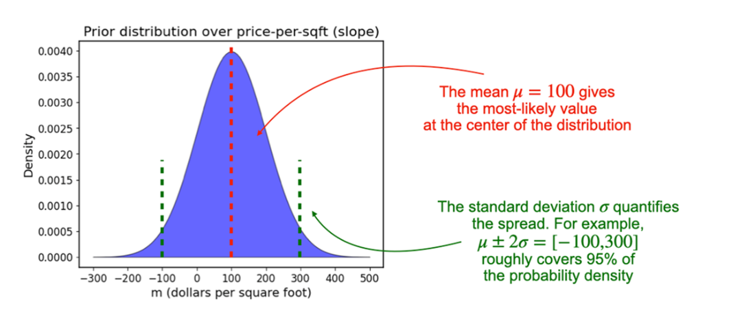
The bell curve shows why a prior can favor 100 without treating it as a certain answer: its wide spread represents uncertainty. section 3.12
Before using observed prices, check what the prior implies for predictions. Draw possible slopes, multiply each by chosen house areas, and add noise to obtain simulated prices. Inspecting those prices can reveal whether the starting assumptions produce sensible results. section 4.4
from scipy.stats import norm

seed = 0
x = np.linspace(500, 2500, 10)  #A
noise = norm.rvs(
    0,
    20000,
    size=10_000, )                               #B
prior_m_samples = norm.rvs(
    mu,
    np.sqrt(sigma2),
    size=10_000, )
prior_y_samples = (
    prior_m_samples.reshape(-1, 1)
    * x.reshape(1, -1)
    + noise.reshape(-1, 1)
)                               #C
The listing draws 10,000 slopes from the normal prior and uses NumPy array reshaping to calculate predicted prices for ten house areas. section 4.4
A normal prior has a practical limitation: it assigns some probability to negative values. A negative price-per-square-foot slope conflicts with the intended assumption that this slope is non-negative. Raising the mean or reducing the spread makes negative slopes less likely, but cannot exclude them. When the restriction matters, choose a different prior; that may mean giving up a convenient conjugate, closed-form update. section 5.2
Normal priors also describe real-valued centers or effects in more layered models. Standard normal priors can represent cluster centers after data have been standardized; a broad normal prior can represent a hierarchical model’s base effect. Quantities that must stay non-negative, such as cluster widths or an effects spread, instead receive half-normal priors in these examples. section 8.6 section 7.4
