GPipe

As explained in Sutskever's List

GPipe is a system for training neural networks by partitioning computation into pipeline stages across devices.

GPipe introduced pipeline parallelism as a way to train neural networks too large for one device. It partitions a model into stages across devices, then streams micro-batches through those stages so devices work concurrently. section 6.3.1

Two mechanisms address common limits of model parallelism:

• Accumulate gradients across micro-batches and apply one synchronized update per full batch, avoiding stale weights. section 6.3.1
• Use activation checkpointing, or recomputation, to save memory by recalculating selected activations during backpropagation. section 6.3.1

Scaling model capacity

On eight GPUs, GPipe enabled an AmoebaNet with 1.8 billion parameters, compared with about 82 million on one 8-GB GPU. On 128 TPU partitions, the team trained an 83.9-billion-parameter Transformer. section 6.3.2

Figure 6.6 Pipeline parallelism compared to naive model parallelism. (a) A simple neural network partitioned across four accelerators, with forward passes F₀ – F₃ flowing upward and backward passes B₀ – B₃ flowing downward to compute gradients. (b) In naive model parallelism, layers are split sequentially across devices. Because each stage must wait for the previous stage to complete, much of the hardware remains idle, leading to low utilization. (c) Pipeline parallelism mitigates this inefficiency by splitting each mini-batch into smaller micro-batches. These micro-batches flow through the pipeline in a staggered fashion, keeping devices busy by processing different micro-batches simultaneously. While idle-time bubbles still appear during the pipeline “fill” and “drain” phases, overall utilization improves significantly. Gradients are accumulated across micro-batches, and updates are applied synchronously at the end of each full batch. Used with permission granted by the lead author (Yanping Huang).

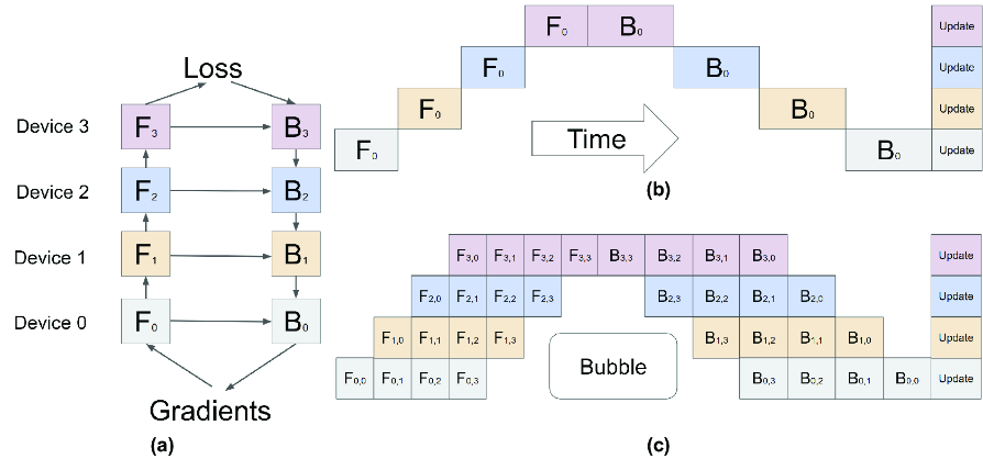
Compare sequential model parallelism, where devices wait on one another, with staggered micro-batches that keep more devices busy; pipeline fill and drain still leave some idle time. section 6.3.1

How Sutskever's List covers it

How deep it goes

Explains staged partitioning, micro-batch scheduling, synchronized gradient accumulation, and activation recomputation, then quantifies results on two architectures.

Examples

Compares an 82-million-parameter AmoebaNet on one 8-GB GPU with larger multi-device AmoebaNet and Transformer experiments.

What you can do after

Evaluate how micro-batches, partition count, and recomputation affect model capacity, throughput, and idle-time bubbles.

How it connects

Connects pipeline parallelism to model parallelism, activation checkpointing, rematerialization, and synchronized gradient updates.

liveBookmanning.com

Read Sutskever's List on liveBook Get the book at manning.com

Also explained in

• 

  liveBookmanning.com
  Designing Deep Learning Systems: A guide for software engineersA pipeline-parallel training implementation that splits batches into microbatches and accumulates their gradients before updating model parameters.

Compare how 2 books explain GPipe →

Related concepts

• pipeline parallelismimplements · Pipeline parallelism is a model-parallel technique that divides sequential computation into stages on different devices and concurrently processes multiple inputs through them.
• AmoebaNetuses · AmoebaNet is a convolutional neural network architecture discovered through neural architecture search for image recognition.

This explainer was generated by Manning's knowledge graph from the text of Sutskever's List. The section links point to the parts of the book it draws on.