A predecessor graph records at most one predecessor for each node. During breadth-first search, each newly discovered node is linked to the frontier node that found it, creating enough history to reconstruct a path without searching again. section 6.1.1 section 6.1.2
A breadth-first search builds and uses the graph in a small sequence:
- Start with the initial frontier, collect neighboring nodes, and remove the current frontier from the searchable graph. section 6.1.1
- Add predecessor edges for the newly discovered nodes, while filtering out nodes already removed from the graph. section 6.1.2
- Stop when the target enters the next frontier; otherwise continue with that frontier. section 6.1.1
- Backtrack from the target through its single predecessor at each step, then reverse the collected nodes to obtain the path. section 6.1.3
Representing the search state
In Haskell, represent the state as a frontier, the remaining graph, and the predecessor graph: `type SearchState a = ([a], DiGraph a, DiGraph a)`. A successful search returns `Successful preds`; an unsuccessful search returns `Unsuccessful`. The path finder follows one child from the target until it reaches the node with no predecessor, then reverses the result. section 6.1.2 section 6.1.3
Figure 6.3 An example of a search on a graph (searching from 1 to 6) and the predecessors being built in every step
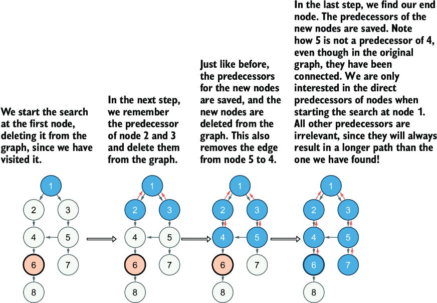
Use the search diagram to follow predecessor edges as the frontier expands from the start toward the target. section 6.1.1
Listing 6.3 Our backtracking algorithm to find a path in a predecessor graph
findSolution :: Eq a => DiGraph a -> [a]
findSolution g = L.reverse (go end)       #1
  where
    go x =
      case children x g of      #2
        [] -> [x]      #3
        (v : _) -> x : go v    #4
Use the backtracking listing to inspect the recursive path reconstruction and its final reversal. section 6.1.3