An integral reverses differentiation—almost. Differentiation removes constants, so integrating a derivative recovers a family of functions rather than one unique original: an additive constant may be missing. For example, differentiating a*x² + b*x + c gives 2*a*x + b, while integrating that result returns a*x² + b*x. Keep the lost constant in mind whenever reversing a derivative. section 5.1.4 section 5.5
Integrals also describe accumulated change geometrically. The difference between an antiderivative at two endpoints gives the signed area between a graph and the x-axis over that interval. This makes an integral useful as a constraint: instead of only matching a function’s values and slopes at selected points, a model can also match the total area across a range. section 7.1.2
Constrain a sine approximation with area
To approximate sine for a simulator, define an odd seventh-degree polynomial in SymPy, differentiate it for slope constraints, and integrate it for an area constraint. Require the polynomial to equal 1 at π/2, have slope 1 at 0 and slope 0 at π/2, and have integral 1 from 0 to π/2. Solving these four equations produces a compact model whose coefficients closely resemble the corresponding sine-series coefficients. section 7.1.2 section 7.1.2
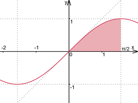
The shaded interval gives the practical reading of a definite integral: the area under sine from 0 to π/2 is 1. section 7.1.2
Polynomial integration stays especially manageable: integrating a polynomial produces another polynomial. Together with derivatives and factorial-scaled coefficients, this supports Taylor and Maclaurin-style reconstruction and approximation. Choose an integral constraint when matching accumulated behavior matters; values and derivatives alone may leave a different approximation with similar local behavior. section 6.2.1 section 7.1.2
