An interpolant is a function whose graph passes through every specified data point. Interpolation is therefore the exact-fitting special case of approximation: with N data points, a polynomial interpolant normally has degree N−1. section 6.3.6 section 6.7
For polynomial data, the Vandermonde matrix is a practical way to compute the coefficients. Least squares can also produce an interpolating polynomial, while Lagrange interpolation makes the idea of basis polynomials especially visible. section 6.3.6 section 6.7
Inverse-distance interpolation
Given points (1, 3) and (3, 1), assign each value a weight inversely proportional to its distance from x, then divide the weighted sum by the sum of the weights. With power n = 1, the resulting interpolant is also linear. At x values approaching 1, such as 1.000001, it approaches 2.99999, demonstrating convergence toward the specified value. The endpoints themselves require separate handling because a weight divides by zero. section 8.3.1
Changing the inverse-distance power changes the interpolant’s shape, and using several points extends the method beyond the two-point case. No single spatial interpolation method serves every need; alternative weight functions, value functions, or more local constructions may be worth exploring. section 8.3.1 section 8.5
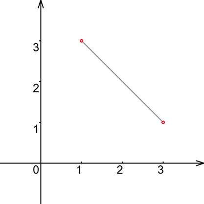
Use the figure to compare the straight-line shape produced by inverse-distance interpolation with power n = 1. section 8.3.1
Figure 8.17 Here is the same interpolation with (from left to right) n = 2, n = 3, and n = 4. Raising the power of n changes the shape of the interpolant.
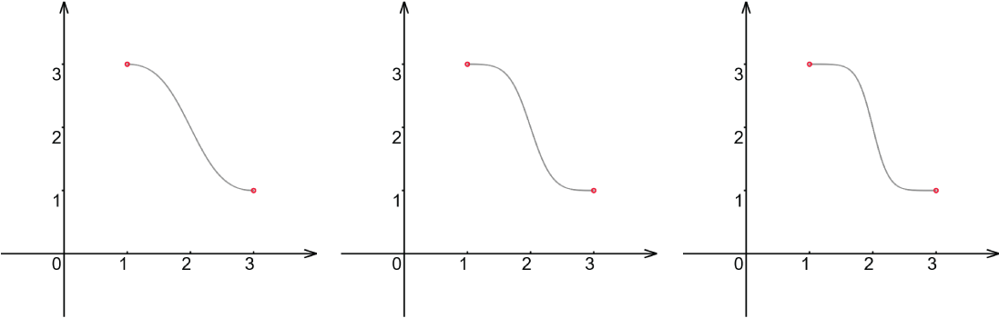
Use the figure to see how powers n = 2, 3, and 4 reshape the same interpolant. section 8.3.1
