A kernel density estimate (KDE) describes where numeric observations are concentrated without requiring one fixed distributional shape. Place a small kernel, such as a Gaussian-shaped curve, at each observation and combine the curves. The resulting density is high where observations gather and low in sparse regions. section 2.1.6
For outlier detection, low density can identify values between groups as well as values beyond the extremes. Consider purchases concentrated near $10 and $500: a $100 purchase may be unusual even though it is not exceptionally small or large. KDE, histograms, and nearest-neighbor calculations can handle such internal outliers more flexibly than tests built around a single average and variance. A low-density value is a candidate for investigation, not proof of a problem. section 2.1.6 section 2.9
Figure 2.8 Given a dataset, here containing 10 points, KDE can estimate the distribution by creating a small kernel—in this case, a Gaussian shape—at each point and summing these. The three panes show the effect of adjusting the widths of the kernel. With narrow kernels, there is less summing of the kernels; the final KDE estimate resembles the individual kernels and fits the data tightly. With wider kernels, the KDE estimate becomes smoother. We wish to find a balance with an appropriate bandwidth. In this case, the first or second panes or somewhere in between may work best.
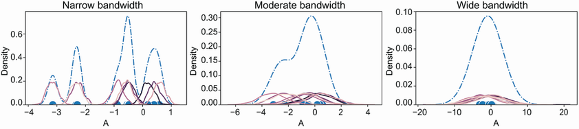
The ten-point illustration shows why bandwidth matters: narrow kernels follow individual observations closely, while wider kernels produce a smoother estimate. Neither extreme is automatically the right fit. section 2.1.6
Score sparse values in one column
For the hue-mean column of the segment dataset, reshape the values into one-column input and fit scikit-learn’s KernelDensity with a Gaussian kernel and bandwidth of 0.2. Score each observation, then flag scores below a threshold set at the first score quartile minus 2.2 times the interquartile range. Plotting the flagged values against a histogram checks whether they lie in sparse regions. The bandwidth and threshold are choices to inspect, not universal settings; seaborn’s histplot with kde=True offers a quick view of the density shape. section 2.1.6
A single density estimate across a whole dataset may be misleading when regions have different densities. One alternative is to cluster the data, estimate density within each cluster, and compare a point’s KDE with the average KDE of its cluster. Ratios make those comparisons more meaningful across clusters than raw scores. Because clustering can change across runs or plausible cluster counts, averaging results from multiple clusterings can improve stability, though it does not remove dependence on clustering quality. section 7.8.2
KDE also has a different use: generating synthetic values that resemble an observed feature’s distribution. Generating features independently this way does not, by itself, preserve associations between columns. For detection through a common interface, PyOD’s KDE detector wraps scikit-learn’s KernelDensity and exposes fitted training scores through decision_scores_. section 11.2.2 section 6.1

