Imagine choosing cloud-service instances for a server with a budget of eight credits. Each instance costs credits and adds processing throughput. Capacity is the hard ceiling: the selected instances may cost eight credits in total, but not nine. The goal is to get the most throughput without crossing that ceiling. section 7.1
A dynamic programming table considers every smaller capacity from zero through the full limit W. Cell T[i, j] holds the best value obtainable from the first i items while using no more than j capacity. The zero-item row and zero-capacity column contain zero. These smaller budgets let the algorithm reuse answers instead of reconsidering every selection from scratch. section 7.1 section 7.4
For each item and capacity, ask whether the item fits:
- If its weight exceeds the current capacity, skip it and copy the value from the row above. section 7.1
- If it fits, compare skipping it with taking its value plus the previous row’s answer for the capacity left over. Using the previous row prevents taking the same item twice. section 7.1
A choice at capacity eight
Suppose the last instance costs five credits and adds six units of value. At capacity eight, skipping it gives 10. Taking it leaves capacity three, whose earlier best value is five; 6 + 5 = 11. The better answer is 11, with total cost still within eight credits. section 7.1
Figure 7.3 Visualization of the math used to evaluate cell T[2, 3] (circled in green) on the second row (w2 = 2, v2 = 3). The algorithm resolves a binary choice by executing a maximum value comparison between two paths. The exclusion path inherits the value directly above (T[1, 3] = 2). The active inclusion path accepts the new instance's throughput value (v2 = 3, highlighted in the red solid box) and subtracts its weight from the current capacity (3 - 2 = 1), forcing a pointer lookup to the previous row at column 1 (T[1, 1] = 2, highlighted by the red dotted circle). The combined value of 5 outperforms the exclusion path, updating the cell state.
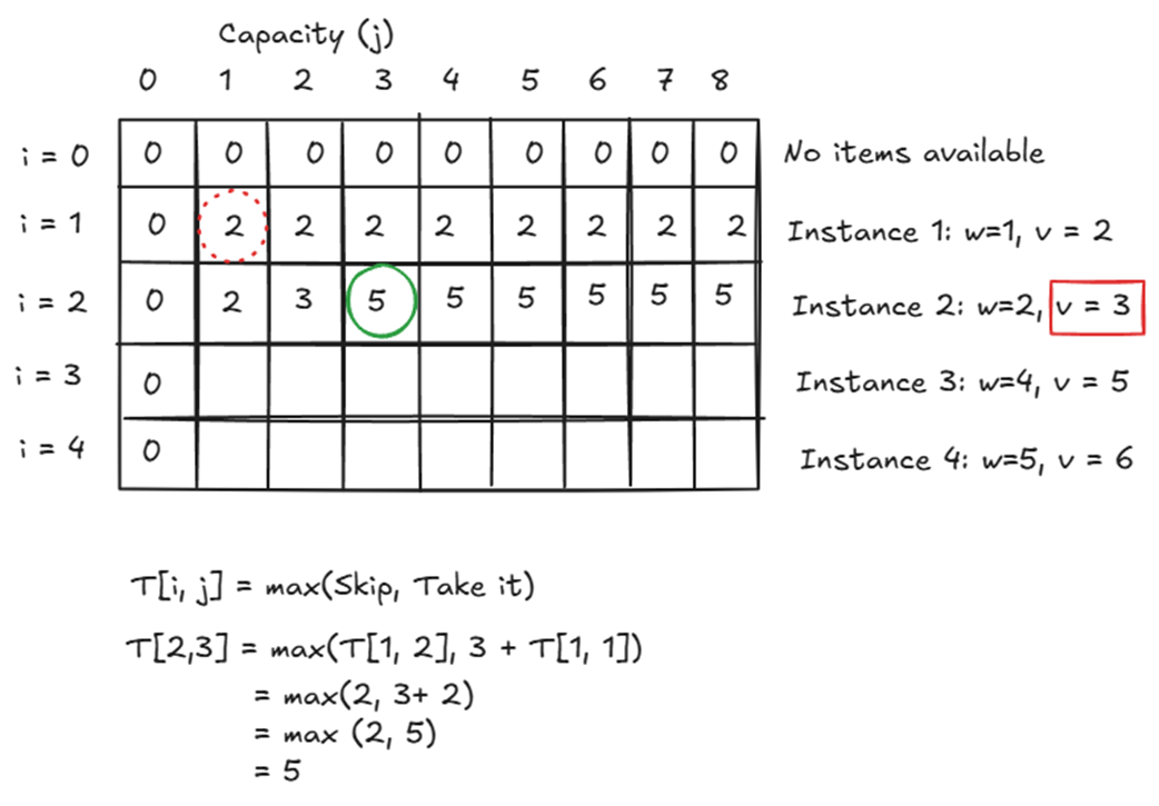
The marked cells show why taking an item means looking up its remaining capacity in the previous row, then comparing that result with skipping it. section 7.1
Capacity also determines the table’s size. With n items and a numeric limit W, the standard table uses (n + 1) × (W + 1) cells and takes O(nW) time and space. Eight credits makes a small table; an enormous numeric limit can make the same approach impractical even with only four items. section 7.3