Markov chain monte carlo

As explained in Machine Learning Algorithms in Depth

Markov chain Monte Carlo is a Monte Carlo methodology that samples a Markov chain to approximate a target probability distribution, typically a posterior distribution.

Markov chain Monte Carlo (MCMC) approximates a posterior distribution p(θ|x) by sampling a high-dimensional parameter space. Construct a Markov chain whose stationary distribution is the target posterior, then let it move through the space. The fraction of time it spends near a state θ reflects that state's posterior probability. Samples from the chain can then support Monte Carlo estimates of quantities of interest. section 1.4.1 section 2.0

The central implementation choice is how to move between states:

• Gibbs sampling updates one variable at a time, drawing from its distribution conditional on the latest values of the other variables. section 2.9
• Metropolis–Hastings proposes a new state x′ from q(x′|x), then accepts or rejects it using a ratio designed to satisfy detailed balance. section 2.9

From direct sampling to high-dimensional sampling

For an exponential random variable, direct sampling starts with u drawn uniformly from (0, 1) and transforms it to −ln(1 − u)/λ using the inverse cumulative distribution function. High-dimensional posteriors motivate a different approach: construct a chain that spends more time where the target posterior is more probable. Monte Carlo exercises such as estimating π, a binomial tree model, and a self-avoiding random walk provide practice with simulation before the sampling algorithms. section 1.4.1 section 2.0

Figure 1.6 Exponential RV probability density function (left) and cumulative density function (right)

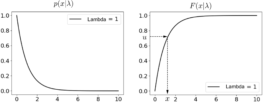
The exponential density and cumulative distribution illustrate the low-dimensional inverse-CDF method used as a contrast to sampling a high-dimensional posterior. section 1.4.1

MCMC belongs to the sampling approach to Bayesian inference. Variational inference instead chooses a tractable distribution and optimizes its fit to the posterior. Sampling can apply to a broad range of problems, including those without convenient conjugate priors; variational inference is often faster on small to medium problems and has a more straightforward stopping decision. section 1.4.1 section 4.3

How Machine Learning Algorithms in Depth covers it

How deep it goes

Defines the stationary-distribution principle and sketches Gibbs and Metropolis–Hastings updates without specifying a complete sampler implementation.

Examples

Uses inverse-CDF exponential sampling, π estimation, a binomial tree model, and a self-avoiding random walk as sampling examples.

What you can do after

Evaluate/understand it as a way to estimate posterior quantities and distinguish sampling from variational approximation.

How it connects

Connects Markov chains and Monte Carlo integration to Gibbs sampling, Metropolis–Hastings, probabilistic graphical models, and variational inference.

liveBookmanning.com

Read Machine Learning Algorithms in Depth on liveBook Get the book at manning.com

Also explained in

• 

  liveBookmanning.com
  Causal AIMarkov chain Monte Carlo is a family of sampling algorithms that generate a Markov chain whose limiting distribution is a target probability distribution.

Compare how 2 books explain markov chain monte carlo →

Related concepts

• metropolis-hastings samplingincludes · Metropolis-Hastings sampling is a Markov chain Monte Carlo method that proposes state changes and accepts or rejects them probabilistically to generate samples from a target distribution.
• stochastic variational inferencealternative to · Stochastic variational inference is a variational inference technique that optimizes an objective using stochastic estimates, often computed from randomly sampled data subsets.
• variational inferencealternative to · Variational inference is an approximate inference technique that optimizes a tractable family of probability distributions to approximate a target distribution, often a posterior.
• posterior probabilityuses · A posterior probability or distribution expresses the probability assigned to an event, hypothesis, or unknown quantity conditional on observed evidence and prior information.
• Markov chainuses · A Markov chain is a stochastic process of states whose transition probabilities depend on the current state rather than the full preceding history.
• gibbs samplingincludes · Gibbs sampling is a Markov chain Monte Carlo technique that repeatedly samples each variable from its conditional distribution given the others.

This explainer was generated by Manning's knowledge graph from the text of Machine Learning Algorithms in Depth. The section links point to the parts of the book it draws on.