Mathematical function

As explained in Geometry for Programmers

A mathematical function is a relation that assigns exactly one output to each input in its domain.

A mathematical function is a rule that gives every allowed input exactly one output. Think of it as a dependable geometric machine: supply a coordinate, vector, or point, and it returns the result specified by its rule. A pure programming function is a close practical analogy because it accepts input, returns output, and has no other effects. section 2.4.1

The allowed inputs form the domain; the declared output set is the codomain. The outputs actually produced are the range, which may be smaller than the codomain. For sine, every real x has one y, while the outputs stay between -1 and 1. Reversing that relation fails the function test: one y can correspond to infinitely many x values. section 2.4.1

Figure 2.20 The sine function: y = sin(x)

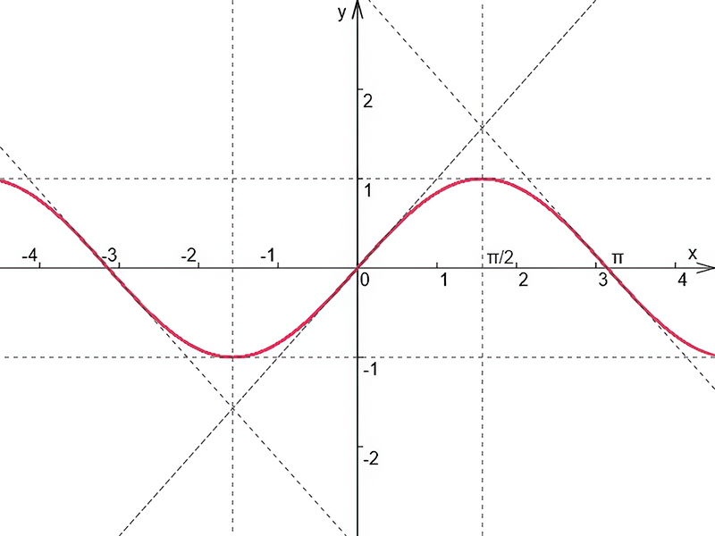
Use the sine graph to see one output assigned to each real input, even though many inputs can share an output. section 2.4.1

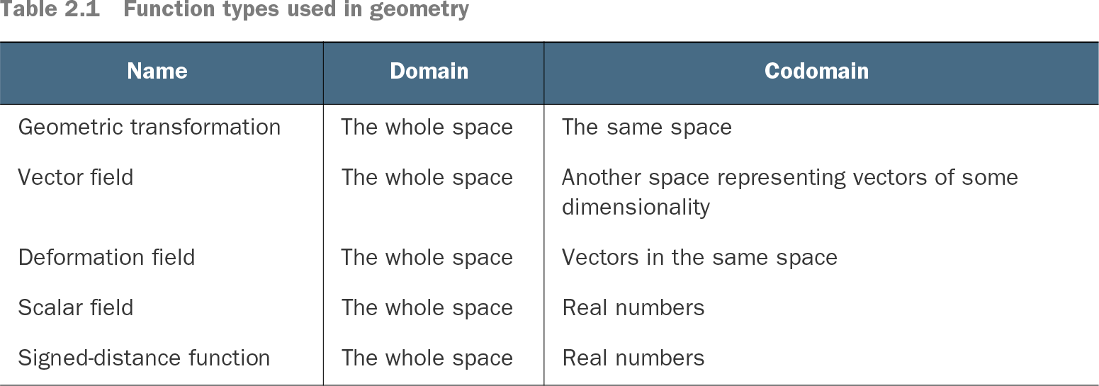
In applied geometry, function types are distinguished by what they accept and return:

• A geometric transformation maps points in a space to points in that same space; applying it point by point describes a change to the whole space. section 4.1
• A vector field maps locations to vectors, while a deformation field maps locations to vectors in the same space. section 2.4.3
• A scalar field and a signed-distance function map locations to real numbers. section 2.4.3

Continuity is an especially useful property when functions model curves and surfaces. A function can be defined everywhere yet still be discontinuous, while smooth continuous functions support measurements of growth, tangent direction, and curvature through derivatives. section 2.4.3 section 5.0

From a circle formula to array-ready code

A circle signed-distance function can be written as d = (x² + y²)^0.5 - 1, then packaged as a Python function of x and y. With NumPy, ordinary numeric expressions often work on arrays directly; a function containing an if may need @np.vectorize so it can process each array element. This is convenient, but vectorized branching addresses array inputs rather than changing the mathematical rule. section 10.1.2

Functions also turn sampled artifacts into geometry. Pixel values can first be represented by a discontinuous function, then interpolated into a smooth continuous one. After shifting it into a quasi-signed-distance function, an iterative fit can place a contour on a threshold isoline, and cubic segments can smooth that contour. section 12.4.5

Table 2.1 Function types used in geometry (view table figure)

Name	Domain	Codomain
Geometric transformation	The whole space	The same space
Vector field	The whole space	Another space representing vectors of some dimensionality
Deformation field	The whole space	Vectors in the same space
Scalar field	The whole space	Real numbers
Signed-distance function	The whole space	Real numbers

Compare common geometry-oriented function types by their domain and codomain. section 2.4.3

How Geometry for Programmers covers it

How deep it goes

Defines functions through relations, domain, codomain, range, and inverse sine, then applies their types and properties in geometry.

Examples

Uses sine and its inverse relation, a circle signed-distance expression, NumPy vectorization, and pixel-image interpolation into a smooth contour.

What it assumes

Builds from familiar programming-function intuition while introducing relations, domains, codomains, and ranges through sine.

What you can do after

Apply it via Python, SymPy, and NumPy to express geometric rules and process scalar or array inputs.

How it connects

Connects functions to relations, domain, codomain, range, continuity, geometric transformations, vector fields, scalar fields, and signed-distance functions.

liveBookmanning.com

Read Geometry for Programmers on liveBook Get the book at manning.com

Also explained in

• 

  liveBookmanning.com
  Unit Testing Principles, Practices, and PatternsA mathematical function is a computation that maps each input to exactly one output without hidden inputs or outputs and produces the same output for a given input.

Compare how 2 books explain mathematical function →

Related concepts

• geometric transformationincludes · A geometric transformation is a mapping or operation that changes or expresses the position, orientation, scale, shape, or coordinate representation of geometric objects.
• sine functionincludes · The sine function is a periodic trigonometric function that maps a real number or angle to a value between −1 and 1.
• relationkind of · A relation is a rule or set of associations that links elements of one set with elements of another set without requiring unique outputs.
• functional, stateless philosophyused by · Functional programming is a programming paradigm that expresses computation through the evaluation and composition of functions, typically favoring immutable data and minimizing mutable state and side effects.
• polynomial functionincludes · A polynomial function is a function expressible as a finite sum of constant multiples of nonnegative integer powers of one or more variables.

This explainer was generated by Manning's knowledge graph from the text of Geometry for Programmers. The section links point to the parts of the book it draws on.